This article is the third part of a mini-series on structuring and executing machine learning projects with a core focus on deep learning. (The earlier two articles are How to plan and execute your ML and DL projects and Becoming One With the Data.) This article’s aim is to discuss several aspects of training neural networks in a methodical way in order to minimize overfitting and develop a checklist of the steps that make that possible.

One of the key elements that ensures a network is training in the way it should is its configuration. As Jason Brownlee of Machine Learning Mastery states, “Deep learning neural networks have become easy to define and fit, but are still hard to configure.”

This article is divided into the following sections:

• Training a neural network, which will discuss what to keep in mind before starting the training process to have better control over our models.
• Gradually increasing model complexity (if needed), where we will see why it is important to start with a simple model architecture and then ramp up the complexity as needed.
• Tuning the knobs, which will deal with the process of hyperparameter tuning to enhance the performance of a neural network.
• Going beyond with ensembling, knowledge distillation, and more, which will discuss techniques like model ensembling and model compression.

Along the way, I’ll share personal commentary, stories from established deep learning practitioners, and code snippets. Enjoy!

Training a Neural Network

Neural networks act weird sometimes it can get really difficult to trace back to the reasons. So, in this section, let’s start by looking at the common points that can fail a neural network.

Implementation Bugs:

• What if while loading image data, you accidentally jumbled up the order of the images and labels, and all of the images got labeled in the wrong way? You might not be able to spot it instantaneously, since a few (image, label) pairs may be correct by chance. Consider the following code snippet:

X_train = shuffle(X_train)
Y_train = shuffle(y_train)

       
 Whereas it should be:

X_train, y_train = shuffle(X_train, y_train)

• What if you standard-scaled the categorical features of a tabular dataset? Representing categorical features as one-hot encoded vectors and treating them as just another numeric features are drastically different. Consider the following mini dataset:

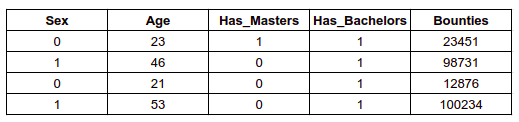
  There are three categorical features here: Sex, Has_Masters, and                   Has_Bachelors. You may one-hot encode to better represent the relationship or you may just keep them as they are. There are two continuous features in the dataset: Age and Bounties. They vary largely in scale, so you would want to standardize their scales. Since all of the variables are numerical, you may think to use the following to standardize the continuous features:

scaler = StandardScaler()
scaled_train = StandardScaler().fit_transform(data.values)

But it should be:

scaled_train = StandardScaler().fit_transform(data[non_cat_feats].values)

• What if you initialize all the weights to zero and then use ReLU?

There are several ways to initialize the weights in a neural network. You can start with all zeros (which isn’t advisable, and we will see it a second), you can randomly initialize them, or you can choose a  technique like Xavier initialization or He initialization. If you go with the Xavier or the He scheme,  you need to think about the activation functions accordingly. For example, the Xavier scheme is recommended for tanh activations and the He scheme is recommended for ReLU activations. Consider the following example while declaring your network using Keras:

# Define a Sequential model
model = Sequential()
model.add(Dense(64, kernel_initializer='zeros', activation='relu'))
...

In the above example, the model’s weights are initialized to zero, which means that after multiplying the inputs to the zero-initialized weights, there’ll be only zeros. That passes through the ReLU activation function to yield zeros, too. A better way to do this if you want to use the ReLU activation function would be:

# Define a Sequential model
model = Sequential()
model.add(Dense(64, kernel_initializer='he_normal', activation='relu'))
...

• Are you using PyTorch and have you forgotten to zero the gradients? This is specific for PyTorch users, since those gradients are accumulated during backpropagation and are not updated. You don’t want to mix up the weights in mini-batches; you want the parameters to be updated in the correct way.

    Consider the following training loop in PyTorch:

for e in range(epochs):
    running_loss = 0
	# Loop over the images and labels in the current batch
    for images, labels in trainloader:
    # Load the data to the available device and reshape the images           
        images = images.to(device) 
        labels = labels.to(device)
        images = images.view(images.shape[0], -1)
               			
        # Get predictions from the model and determine the loss
        log_ps = model(images)
        loss = criterion(log_ps, labels)

        # Calculate the gradients and update the parameters
        loss.backward()
        optimizer.step()

        running_loss += loss.item()

Notice that the code does not zero out the gradients before updating the           parameters. Try instead the following line of code just before you employ the           model to get the predictions: optimizer.zero_grad().

Model’s Sensitivity Towards Hyperparameter Choices:

• Using a very high learning rate at the very beginning of the training process. You wouldn’t want to diverge at the very beginning of the training process, nor would you want to have a too-small learning rate such that the model takes forever to get trained.

 A very high learning rate can result in very large weight updates, causing it to         take NaN values. Due to this numerical instability, the network becomes totally           useless when NaN values start to creep in.

 There’s a whole area of learning rate annealing to dive into; if you’re interested,       start with this article.

• Setting too few epochs to properly train a model on a large dataset. You may have a decently large dataset—for example, ImageNet—and you are not letting the model (not a pre-trained one) go through the data for a sufficient amount of iterations.
• Setting too large of batch size for a relatively small dataset. You are fitting a model with only 100 images and you are setting a batch size of 64. In cases like this, having a relatively smaller batch size helps.

Dataset Construction and others:

• You did not construct the validation set in the right way. The class distribution in the training dataset varies largely from the validation set. There can be a problem with the validation itself as well. Say you are building an image segmentation model and the dataset consists of several frames snapped out of videos. Creating a partial validation set with random splits might not be a good idea, since you may end up having an image(s) in the validation set that is very contiguous to another image in the training set. In that case, it would be very easy for the model to do the segmentation on the image from the validation set. A good validation set contains images that are non-contiguous in nature with the images in the training set. (That example is inspired by this lesson of the course Practical Deep Learning for Coders v3 offered by fastai.)

• The distribution of the data in the train set is largely different from the test set. For example, you’ve trained your model on low-resolution images of cats and dogs and you are testing the model on high-resolution pictures. Consider the following example to understand this more clearly:

Consider an imaginary network being trained on a dataset consisting of left-side images. Now that trained network is very likely to fail if it is tested on the right-           side images as the network never got to see any image of cats with different             colors other than black.

• There’s label noise in the dataset. This is a very severe problem and hard to detect. This problem happens when the data points are labeled incorrectly. Suppose you are dealing with the Dogs vs. Cats dataset and there are a few images of dogs that are mistakenly labeled as cats and vice-versa. If you train a model with the errors unfixed, you’ll find it doesn’t perform as you intended.
• Suppose you are fine-tuning a pre-trained model to classify different breeds of goldfish. If while constructing the dataset, you didn’t normalize the dataset with the mean and standard deviation of the original dataset on which the pre-trained model was trained. This way, your network will not be able to capture the true distribution of the dataset it is being trained on.
• There’s a major class imbalance in the dataset, but you got a pretty good accuracy score and you fall prey to the accuracy paradox. When the model is deployed, it fails to detect the minor classes.

The above problems are the most common ones encountered in the day-to-day work of deep learning practitioners. There’s a strong need for us to fully own our deep learning models so that we can debug them as needed without losing our sanity.

What makes the whole deep learning model debugging process very hard is the fact that a deep learning model can fail silently. Consider the following instances:

• During the data augmentation process, your hyperparameter choices augment an image in such a way that its label changes.

• While applying transfer learning, you didn’t use the mean of the original dataset on which the model (that was to be used) was trained to perform mean subtraction with your custom dataset. Imagine you are using a VGG16 network to build an image classifier with the Dogs. vs. Cats dataset and the network was trained on the ImageNet dataset. Now let’s say you’re writing the data loader like the following:

# initialize the data generator object
datagen = ImageDataGenerator()

# specify the mean to the data generator object
# so that it can perform mean subtraction on the fly
datagen.mean = dogs_cats_mean

But the correct way, in this case, would be:

# initialize the data generator object
datagen = ImageDataGenerator()

# specify the mean to the data generator object
# so that it can perform mean subtraction on the fly
mean = np.array([123.68, 116.779, 103.939], dtype="float32") # ImageNet mean
datagen.mean = mean

The above snippets use the Keras ImageDataGenerator class to stream the data to the model.

Unfortunately, these things are not trivial to unit-test, either. You’ll want to have full command over the model, its configurations, the hyperparameter choices, and so on to understand why it fails and why it performs well. As Andrej Karpathy explains:

As a result, (and this is reeaally difficult to over-emphasize) a “fast and furious” approach to training neural networks does not work and only leads to suffering. Now, suffering is a perfectly natural part of getting a neural network to work well, but it can be mitigated by being thorough, defensive, paranoid, and obsessed with visualizations of basically every possible thing.

Clearly, we need a decent level of expertise in the subject to enable us to spot the above kinds of problems at the right time. This comes with experience, knowledge, and deliberate practice.

As we practice, we’ll need to know some of the most common strategies to not cause ourselves the pain of wonky model weirdness. Training neural networks involves a generous amount of prototyping. Rapid prototyping without enough carefulness might result in a loss of useful components developed during the prototyping process. In the next section, we will focus on some of the important aspects of the model prototyping process and some strategies to apply.

Maintaining a Healthy Prototyping Process

Deep learning experiments involve rapid prototyping, i.e. trying out new model architectures for the given task, trying out different configurations with the same model architecture, and so on. Matt Gardner et. al. have meticulously enlisted three main goals of prototyping in their widely popular deck Writing Code for NLP Research, and I’ll summarize them below.

• Write code quickly: Set up a baseline by reusing existing code/frameworks (aka: don't reinvent the wheel!). Try to find an existing project which solves the same problem (or something that closely resembles the problem) you are working on. The idea here is to get away from the standard bits quickly and focus more on the novel bits in the prototyping process.

It is also advisable to use someone else’s components carefully. You should be able to read the code, you should be able to bypass the abstractions whenever needed, and so on.

• Run experiments and keep track of what you tried: Sometimes it becomes almost impossible to keep track of everything that is happening during the prototyping process if you and your team do not maintain a register accordingly. As a result, you might miss out on something incredible that happened during the prototyping process. Summarize the experiments during the prototyping process along with the suitable metrics in a platform like FloydHub or a spreadsheet with git commits and their results. The following figure represents this idea beautifully:

• Analyze model behavior. Did it do what you wanted? Is your north star metric improving? If not, then figure out why. A good starting point is to analyze the bias-variance decomposition happening within the network. TensorBoard can be a big help, as it enables you to visualize the training behavior of your network very effectively with a number of customization options. Iterate on the hidden spots of your data as suggested in Becoming One With the Data article.

Now, we’ll discuss a very crucial sanity-checking mechanism that can help in identifying a lot of hidden bugs in a model and sometimes in the data preprocessing steps as well.

Overfitting a Single Batch of Data

This technique assumes that we already have a model up and running on the given data. Now, we want to be able to get the loss arbitrarily close to zero on a single batch of data. This brings up a number of issues:

• The loss could go up instead of down
• The loss could go down for a while, then explode
• The loss could oscillate across a region
• The loss could get down to a scalar quantity (0.01, for example) and not get any better than that

Here is a collection of the most common causes that can result in the above-mentioned issues:

In my experience, I’ve found my most common mistakes are either not loading the data and the labels in the correct order or not applying softmax on the logits.

Next up, we’ll discuss why it often helps to start with a simple model architecture for an experiment and then gradually ramp up the complexity. It’s not only helpful for better research but is also tremendously effective for model debugging purposes.

Model Complexity as a Function of Order

Starting simple is more important than we think. Fitting a shallow fully connected network to our dataset is bound to give us poor performance. We should be sure about this part and it shouldn’t deviate much. If it does, there’s definitely something wrong. Detecting what’s wrong in a simpler model is easier than in a ResNet101 model.

Before reusing a pre-trained model, determine if that model is really a good fit for the task at hand. The following are a few of the metrics that should be taken into account when choosing a network architecture:

• Time to train the network
• Size of the final network
• Inference speed
• Accuracy (or other suitable metrics that are specific to the task)

P.S.: We used the FashionMNIST dataset in the previous article, and we’ll be using that dataset here as well.

You can follow along with the code shown in the following sections by clicking on this button:

The FashionMNIST dataset comes with predefined train and test sets. We will start by creating smaller subsets of the data including only 1,000 (with 100 images per class) images in the training set and 300 (with 30 images per class) in the test set in random order. We’ll also make sure that there isn’t any skew in the distribution of the classes in both of the sets.

We can first generate a set of random indexes with respect to the labels and the sets with the following helper function:

def generate_random_subset(label, ds_type):
    if ds_type == 'train':
        # Extract the label indexes
        index, = np.where(y_train==label) 
        index_list = np.array(index)
        # Randomly shuffle the indexes
        np.random.shuffle(index_list)
        # Return 100 indexes
        return index_list[:100]

    elif ds_type == 'test':
        # Extract the label indexes
        index, = np.where(y_test==label) 
        index_list = np.array(index)
        # Randomly shuffle the indexes
        np.random.shuffle(index_list)
        # Return 30 indexes
        return index_list[:30]

We can then create the train and tests in an iteratively way, as shown below:

# Generate the training subset
indexes = []
for label in np.unique(y_train):
    index = generate_random_subset(label, 'train')
    indexes.append(index)

all_indexes = [ii for i in indexes for ii in i]

x_train_s, y_train_s = x_train[all_indexes[:1000]],\
            y_train[all_indexes[:1000]]

The training subsets are now created. The test subsets can be created in a similar way. Just be sure to pass test to the generate_random_subset() function when you are creating the test subset.

The two subsets are now ready. We can now blow the whistle and fit a very simple, fully connected network. Let’s start with the following architecture:

The Flatten layer to turn the images into flattened vectors, then a dense layer and finally another dense layer that will produce the output. Let’s look at the code for knowing the other details:

# Baseline model
model = tf.keras.models.Sequential([
  tf.keras.layers.Flatten(input_shape=(28, 28)),
  tf.keras.layers.Dense(128, activation='relu',kernel_initializer='he_normal'),
  tf.keras.layers.Dense(10, activation='softmax')
])

model.compile(optimizer='adam',
              loss='sparse_categorical_crossentropy',
              metrics=['accuracy'])

A straight forward model configuration with He initialization to initialize the weights in the dense since there is a ReLU activation. Check this lecture out if you want to know more about weight initialization in neural networks. It’s time to go ahead and train this little one for 5 epochs and with a batch size of 32 and at the same time validate it -

# Train the network and validate
model.fit(x_train_s, y_train_s,
           validation_data=(x_test_s, y_test_s),
           epochs=5,
           batch_size=32)

And as expected, it didn’t get a score that is worth a like on Social Media:

The model overfits - take a look at the loss and val_loss metrics. Let’s cross-check a few points from the list of the most common bugs in deep learning:

• Incorrect input to your loss function - this is not there in our model since we are using CrossEntropy as the loss function and it handles this situation implicitly. If we were using NegativeLogLoss, we could double-check.
• Numerical instability - inf/NaN - this can be verified by looking at the kind of mathematical operations performed at each layer. Operations such as division, exponentiation, logarithm can lead to inf/NaN. In our case, apart from the last layer.

A few points to consider here:

• Create the random subsets a few times and look out for any peculiar changes in the evaluation metrics. If that is observed we should definitely investigate further.
• Predict on a few individual test samples and manually verify them. If the model classifies an image incorrectly, go for a human evaluation - could you classify that image correctly?
• Visualize the intermediate activations of the model. This helps tremendously in learning how the model is looking at the images. As Andrej Karpathy states in his article:

visualize just before the net. The unambiguously correct place to visualize your data is immediately before your y_hat = model(x) (or sess.run in tf). That is - you want to visualize exactly what goes into your network, decoding that raw tensor of data and labels into visualizations. This is the only “source of truth”. I can’t count the number of times this has saved me and revealed problems in data preprocessing and augmentation.

Let’s go for the second point and make a few predictions. I’ve created a helper function that will take an index as its input and will return the model’s prediction on the image corresponding to the index along with its true label. Here’s the helper function:

def show_single_preds(index):
    pred = model.predict_classes(np.expand_dims(x_test_s[index], axis=0))
    print('Model\'s prediction: ',str(class_names[np.asscalar(pred)]))
    print('\nReality:', str(class_names[y_test_s[index]]))
    plt.imshow(x_test_s[index], cmap=plt.cm.binary)
    plt.show()

Here are some predictions with the function:

• show_single_preds(12)

• show_single_preds(32)

The model makes some incorrect predictions as well:

• show_single_preds(101)

• show_single_preds(45)

Note that the images can vary when you run these experiments since the subsets are randomly constructed.

From the two incorrect predictions, you can notice that the model confuses between Trouser and Dress. The immediate above figure looks much like a trouser for a first glance, but if looked closely it is a dress. This simple model is unable to find out this fine-grained details. Plotting the confusion matrix should shed some light on this:

The model confuses the most in between Pullover and Coat. If anyone’s interested, here’s the code to generate a confusion matrix plot like the above:

# Plotting model's confusion matrix
import scikitplot as skplt

preds = model.predict_classes(x_test_s)

skplt.metrics.plot_confusion_matrix(y_test_s, preds, figsize=(7,7))
plt.show()

The scikitplot library makes it super easy to generate confusion matrix plots.

We are now confident with the baseline model, we know its configurations, we know about its failures. The baseline model takes flattened vectors as its inputs. When this comes to images, the spatial arrangement of the pixels gets lost because of flattening them. This solidifies the ground that it is important to the data representation part mind before feeding the data to the network and this representation varies from architecture to architecture. Although we saw it in examples of images, the general concept remains the same for other types of data as well.

You might want to save the current subset of the training and test sets you are working to see any further improvements when more complex models will be incorporated. Since the subsets are nothing but numpy arrays, you can easily save them in the following way:

# Saving the subsets for reproducibility
np.save('tmp/x_train_s.npy', x_train_s)
np.save('tmp/y_train_s.npy', y_train_s)
np.save('tmp/x_test_s.npy', x_test_s)
np.save('tmp/y_test_s.npy', y_test_s)

numpy.save() serializes the numpy arrays in .npy format. To load and verify if the serialization was done properly we can write something like:

# Load and verify
a = np.load('tmp/x_train_s.npy')
plt.imshow(a[0], cmap=plt.cm.binary)
plt.show()

You should get an output similar to this:

At this point, you can safely proceed towards building more complex models with the dataset. Josh Tobin has listed common architectures in his field guide of Troubleshooting Deep Neural Networks:

Once we have the complex model up and running and we have verified the results it yielded, the next step to follow is to tune the hyperparameters.

Tuning the knobs: Chasing hyperparameters

Hyperparameters have a major impact on a model’s performance. These are things that are specified explicitly by the developers and are not generally learned, unlike weights and biases. In neural networks, examples of hyperparameters include learning rate, number of epochs, batch size, optimizer (and its configurations too) etc. I highly recommend this article by Alessio of FloydHub if you want to deepen your understanding of hyperparameters and several processes to tune them.

We will begin this section by discussing the use of declarative configurations in deep learning experiments. We will then take the most important set of hyperparameters (which varies from network types) and discuss the strategies to tune them in effective ways.

Introduction to Declarative Configuration

Machine learning codebases are generally very error-prone and neural networks can fail silently. Deep learning experiments contain a generous number of trial-and-error-based manual checks with hyperparameters. The choice of hyperparameters becomes more mature as we keep on experimenting with models—the more, the better. We may wish to try out our favorite pairs of batch size and number of epochs or a different set of learning rates or combine them both. We often want to be able to tweak an arbitrary combination of hyperparameters in our experiments.

In these cases, it’s, therefore, a good idea to keep the hyperparameters’ specification section separate from the training loop. There are many frameworks that follow declarative configurations such as TensorFlow Object Detection API (TFOD), AllenNLP, Caffe, and so on. The following figure presents a portion of such a configuration that is followed in TensorFlow Object Detection API:

Notice how the TensorFlow Object Detection API allows us to specify hyperparameters like batch size, optimizer, and so on.  It’s better to design the codebase so that it uses declarative configuration to handle the specification of hyperparameters. I strongly encourage you to check this article to learn more about the TensorFlow Object Detection API.

Organizing the Process of Hyperparameter Tuning

As mentioned earlier, with experience and a good understanding of the algorithmic aspects of the different components, you can get good at choosing the right set of hyperparameter values. But it takes a while to get into that zone. Until you’re there, lean on hyperparameter tuning methods like grid search, random search, coarse to find search, and Bayesian hyperparameter optimization.

In his field guide, Josh has listed out the most common hyperparameters to care about and their effect on model’s performance:

Note that for sequence-based models, these hyperparameters may change.

In the last and final section of the article, we’ll discuss two strategies that work really well when it comes to enhancing the model’s accuracy: model ensembling, knowledge distillation, and more.

Going beyond with Ensembling, Knowledge Distillation, and more

In this section, I’ll introduce you to model ensembling and explain why it works (and when it doesn’t), then tell you about knowledge distillation. But first, let me quote Andrej Karpathy again:

Model ensembles are a pretty much guaranteed way to gain 2% of accuracy on anything. If you can’t afford the computation at test time, look into distilling your ensemble into a network using dark knowledge.

Model Ensembling

The idea of model ensembling is simpler than it sounds; it refers to combining predictions from multiple models. But why do that? Well, neural networks are stochastic in nature, meaning that if you run the same experiments with the same dataset, you may not get the same results all of the time. This can be frustrating in production settings or even in hackathons and personal projects.

A very simple solution to this problem is as follows:

• Train multiple models on the same dataset
• Employ all of those models to make predictions on the test set
• Average out those predictions

This method not only allows the ensemble of different models to capture the variance of the dataset. It also results in a better score than any single model. Goodfellow et. al explains simply why this works in their widely popular Deep Learning book:

The reason that model averaging works is that different models will usually not make all the same errors on the test set.

To learn about different ensembling methods in detail, you can check out this article from the MLWave team.

Model ensembling isn’t the end-all be-all solution; it has an obvious disadvantage when production deep learning systems are concerned, explained below.

A very simple way to improve the performance of almost any machine learning algorithm is to train many different models on the same data and then to average their predictions. Unfortunately, making predictions using a whole ensemble of models is cumbersome and may be too computationally expensive to allow deployment to a large number of users, especially if the individual models are large neural nets, from Distilling the Knowledge in a Neural Network by Hinton et. al.

The heaviness of these models makes it difficult to deploy them on edge devices with limited hardware resources. You might ask, "What if the bulky model can be exposed as a REST API on the cloud and be consumed later on as needed?" But there’s a constraint: lack of reliable internet connection. Then there’s another factor to consider, which is that less complex models are often incapable of capturing the underlying representations of the data. There are also environmental costs to consider when scaling up these models, as well as dependency on the Service-Level Agreement (SLA) if the model serves real-time inference. Even if you have a tremendous connection, it's unlikely that you will deploy the model in the Cloud. e.g. Tesla Autopilot. The car will not be able to always query a cloud service to get its required prediction while it is driving. Such predictions tasks may include object localization, lane detection, pedestrian detection, and so on.

Remember, the larger the network, the more memory it takes up on the device, and the more memory it takes up in the device, the harder it is to deploy it. - Jack Clark - ImportAI 162

We want to be able to distill the knowledge of the complex (heavyweight) models into simpler ones, and we want those simpler models to be good at approximating the relationships learned by the complex models. Hence, it’s time to discuss knowledge distillation.

Knowledge Distillation

The idea of knowledge distillation was first proposed by Hinton et. al back in 2015 in their seminal paper Distilling the Knowledge in a Neural Network. The idea involves two networks: a teacher network and a student network.

The teacher network is employed to extract the patterns from the raw data and it is expected to generate soft targets. The soft targets help us to disambiguate the similarities that may be present in different data points of the dataset. For example, it helps us to understand how many 2s in the MNIST dataset resemble 3. These soft targets come as class probabilities and they capture much more information about the raw dataset than hard targets. The soft targets also denote a sense of uncertainty which is often referred to as dark knowledge.

These soft targets are then fed to the student network to mimic the output of the teacher network (hard targets). The student network is trained to generalize the same way as the teacher by matching the output distribution. But here’s a small catch: the cross-entropy loss is taken over the soft targets (as yielded by the teacher network), rather than the hard targets, which is then transferred to the student network.

I definitely recommend checking this work done by the Hugging Face team that was able to incorporate the idea of knowledge distillation in one of their architectures DistilBERT - a distilled version of the mighty language model BERT.

Lottery Ticket Hypothesis

The size of a neural network depends on the number of parameters it contains. For example, the VGG16 network contains 138 million parameters and its size is approximately 528 MB (Keras). Modern-day language model architectures like BERT and its variants are even heavier. Take a look at the below chart, which shows a gradual increase in the number of parameters in language models.

This heaviness is a major memory constraint for the models when it comes to deploying them for running inference. This is where network pruning techniques come into play; they can reduce the count of parameters in a model by 90% without hurting their performance too much. The concept of Lottery Tickets is an incredible piece of research that explores that phenomenon.  

The idea of deep learning Lottery Tickets was first explored by Jonathan et. al in their 2018 paper The Lottery Ticket Hypothesis: Finding Sparse, Trainable Neural Networks. The authors showed that deleting small weights in a network and retraining them can drive astounding results. The idea they introduced was elegant in its simplicity: train a network, set the weights smaller than some threshold to zero, i.e. prune the weights, and then retrain the network with the unpruned weights to their initial configuration. This led not only to  better performance than the network with no weight pruning; it also showed that:

• Aggressively pruned networks (with 85% to 95% weight pruning) showed no drop in performance compared to the much larger, unpruned network
• Networks that were only moderately pruned (with 50% to 90% weight pruning) often outperformed their unpruned variants

After pruning the weights in the larger network, we get a lucky subnetwork under it which the authors referred to as a winning Lottery Ticket.

For more commentary on Lottery Tickets and how the criteria of pruning weights is decided, definitely check out this article by Uber AI.

Quantization

As mentioned earlier, it’s often unlikely that the final network model will be served as an API via the cloud. In most cases, we want to be able to serve in on-device, like through a mobile phone. Another approach to reduce the size of a heavy model and make it easier to serve is Quantization.

Model quantization is directly related to numerical precision such as Float64, Float32, Float16, Int8, Int16, and so on. Deep learning models generally use Float32 precision in all the computations representing the parameters of the network being the most important ones. The size of a deep learning model is dependent on the precision with which its weights have been recorded. The larger the scale, the heavier the model size becomes. So, the question is: can we leverage lower numerical precision for representing the weights of a (heavy) network? Of course we can, but that comes with the cost of lower accuracy, though it is still comparable to the accuracy yielded by the heavier model. This is achieved through quantization. The below figure shows what happens when the higher precision network weights are quantized to a lower precision.

If you want to learn more about model quantization, start with this article.

Conclusion

You’ve made it to the end: congratulations!

The main purpose behind putting together this article was to accumulate the valuable findings of various researchers in order to give the community one thorough document on everything related to neural networks and their training. We’ve covered how to train a neural network, what bugs you’re likely to find and what to do about them, and the simply brilliant Lottery Tickets. Of course, I couldn’t include everything that is there on this subject of training and debugging neural networks, so look to the links for further reading I included above, and check out these resources for further study, all of which have been foundational to my own understanding of the subject:

• Troubleshooting Deep Neural Networks by Josh Tobin. This is probably the best guide if you want to be truly effective at debugging neural networks.
• A Recipe for Training Neural Networks by Andrej Karpathy, where Andrej shares his personal weapons of choice to train neural networks.
• Improving Deep Neural Networks: Hyperparameter tuning, Regularization and Optimization by deeplearning.ai, a course that teaches many aspects of enhancing the performance of a neural network and covers many fundamental aspects like regularization, hyperparameter tuning, and so on.
• Writing Code for NLP Research, a presentation by Joel Grus, Matt Gardner and Mark Neumann at EMNLP 2018. It discusses a wide range of tips and recommendations that should be kept in mind while writing code for NLP-based applications with research heavily incorporated, and it can easily be extended to deep learning projects in general.
• Reproducibility in ML by Joel Grus, which discusses many critical issues with reproducibility in machine learning and sheds light on a number of solutions to overcome them. This was originally a part of ICML 2019’s Reproducibility in Machine Learning workshop.
• Deep Learning from the Foundations by FastAI, a course that takes an extremely code-heavy approach for teaching deep learning from building blocks.
• Testing and Debugging in Machine Learning by Google Developers, a course that discusses several important aspects starting from debugging your model all the way to monitoring your pipeline in production.
• Better Deep Learning by Jason Brownlee, a book solely dedicated to the theme of improving the performance of deep learning neural network models.
• Toward theoretical understanding of deep learning by Sanjeev Arora, which presents some critical theoretical aspects of deep learning in general and discusses them in detail (this is originally an ICML 2018 tutorial).

But this is not where this series ends. The next article will focus on the joys and tribulations of serving a machine learning model. See you there!

A huge shoutout to Alessio from FloydHub who guided me at each step while writing this article.

FloydHub Call for AI writers

Want to write amazing articles like Sayak and play your role in the long road to Artificial General Intelligence? We are looking for passionate writers, to build the world's best blog for practical applications of groundbreaking A.I. techniques. FloydHub has a large reach within the AI community and with your help, we can inspire the next wave of AI. Apply now and join the crew!

About Sayak Paul

Sayak loves everything deep learning. He goes by the motto of understanding complex things and help people understand them as easily as possible. Sayak is an extensive blogger and all of his blogs can be found here. He is also working with his friends on the application of deep learning in Phonocardiogram classification. Sayak is also a FloydHub AI Writer. He is always open to discussing novel ideas and taking them forward to implementations. You can connect with Sayak on LinkedIn and Twitter.