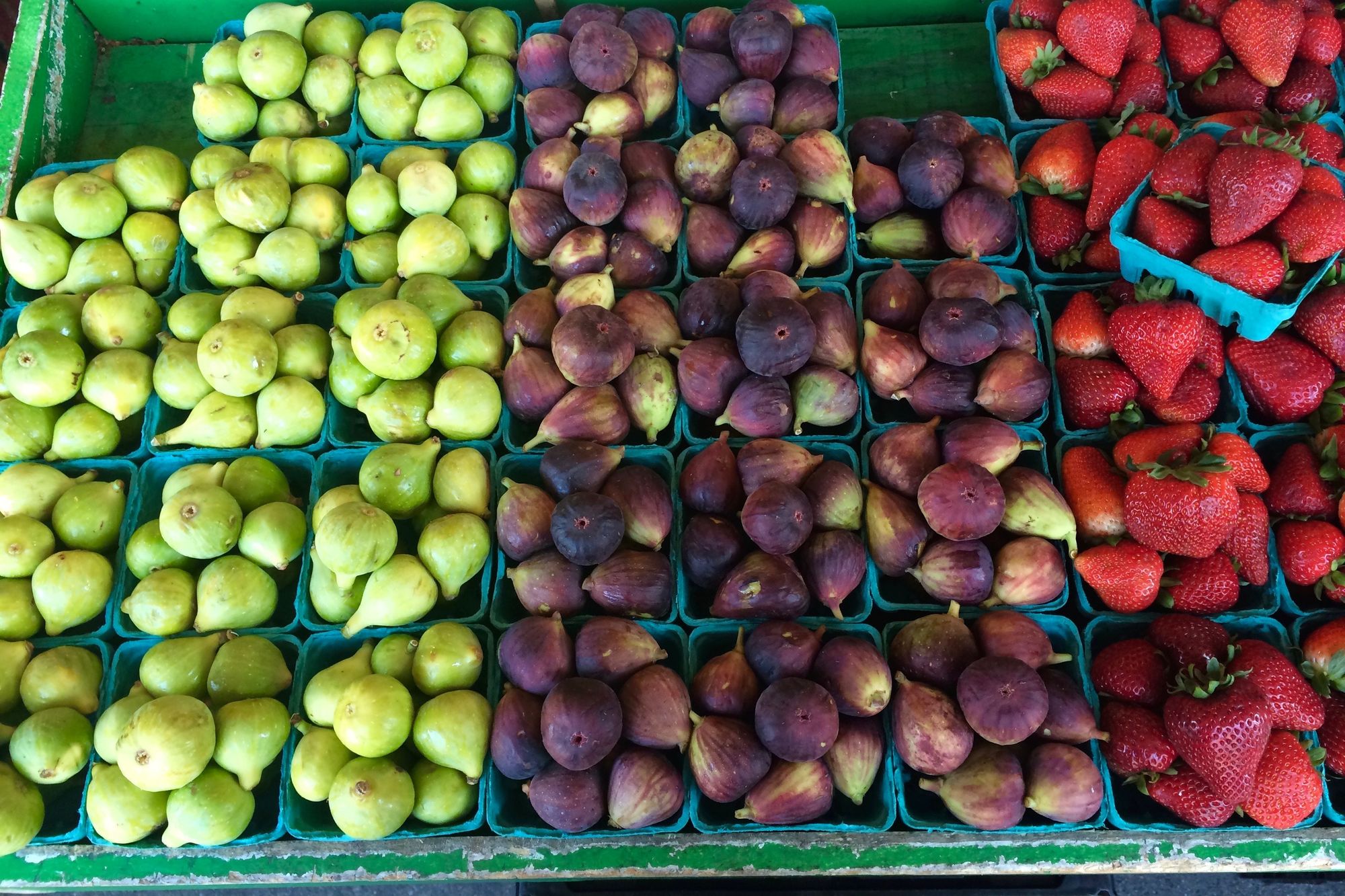
Have you ever organized your bookshelf in a way that the books pertaining to the same subjects are in the same racks or same block? You most likely have. You already know about grouping similar objects together. While the idea is drastically simple, the amount of use cases influenced by this idea is enormous. In machine learning literature, this is often referred to as clustering - automatically grouping similar objects to the same groups.

In this article, we are going to take a look at the old faithful K-Means clustering algorithm which has impacted a very huge number of applications in a wide variety of domains. We will start off by building the general notion of clustering and some of the rules that govern it. We will review some of the different types of clustering briefly and then we will dive into the nitty gritty details of  K-Means. We’ll conclude this article by seeing K-Means in action in Python using a toy dataset. By the time you are done, you’ll have working knowledge of the algorithm and can start applying it to your own use cases.

Sounds interesting? Let’s begin.

Making sense of unsupervised learning

In the world of machine learning, it is not always the case where you will be working with a labeled dataset. Why, you ask? In most of the cases, data is generally labeled by us, human beings. And it is not always possible for us to annotate data to certain categories or classes. Sometimes, the data itself may not be directly accessible. At other times, it may not be very cost-efficient to explicitly annotate data.

Today, the majority of the machine learning world is dominated by a class of algorithms that belong to the family of supervised learning. What if we are in the situation we discussed earlier - we only have the data points but not the category information of them? Unsupervised learning refers to another class of algorithms that try to find the patterns in the data without any explicit labeling.

In one of his keynote addresses (NIPS 2016), Yann LeCun (who is also a Turing awardee) referred unsupervised learning as predictive learning. In predictive learning, a model should be able to approximate any arbitrary part of an input for any amount of observation it is exposed to for that particular input. For example for some input frames in a video, a model should be able to predict the future frame in that video. It is worth noting that this idea governs recent breakthroughs like BERT (by Google), GPT-2 (by OpenAI). These models can perform tasks like predicting the next word, given all of the previous words within some text,  generating conditional synthetic text samples of unprecedented quality and so on. In order to perform tasks like these, these models learn the underlying language distribution. This is useful for a bunch challenging NLP tasks such topic summarization, machine translation and so on.

We now have the main objective that the unsupervised learning algorithms try to cater to. Let’s now discuss a few real-world examples where unsupervised learning can be extremely useful.

Unsupervised learning with (real-world) examples

Assume you have recently founded an online Merchandise company and the business is taking shape at a very fast pace. You have hired a few customer success managers who would be responsible for building and scaling the customer relationship management of your company.

To aid these managers, you have decided to assign different sets of customers to each of them so that they can be more specific in figuring out the strategies business campaigns. Here’s the catch - how would you form these different sets?

All you have is a large pool of the behavioral patterns of the customers which include their browsing patterns, time spent by them at the online portal, their orders and so on. But you do not yet know what might be the possible discrete categories of these customers. All their behavioral patterns might not be the same - some might be similar and some might not. And it is not possible for you to form another team which would manually analyze these patterns and labels them (needs domain expertise which comes at a cost).

The problem is a real one and this is where you can employ unsupervised learning algorithms to automatically group the customers who are very similar in nature. The problem that we discussed just is a very famous problem in the domain of business intelligence. Below are some of the most classic use-cases of clustering:

• Web search: When you search for something with a keyword on the web, think of the amount of information the search engine processes in order to get you a result. Generally, the number of relevant web pages (also referred to as documents) with respect to a particular keyword is huge. Clustering can help to organize these web pages into meaningful groups and thereby enhancing the way the search result is presented.

• Image recognition: Take the example of hand-written digits’ recognition which is like the hello-world problem in the field of computer vision. There exist a wide array of deep neural network architectures which actually beat human-level performance on this task (and similar tasks like this). Now, there can be many shapes of a single digit. The way you write the digit ‘2’ can be largely different from that of mine. It is also practically impossible to collect all these types and train a supervised learning model to recognize them. Clustering can help bypass this problem by automatically grouping these little sub-classes of separate digits and enhance the overall performance of the mother model.

and more.

In this section, we got an idea of some of the problems that are solved by unsupervised learning. We also understood one of the basic themes of unsupervised learning - automatically grouping together the objects that are similar to each other.

Clustering: One entity, different names

We have been discussing clustering since the beginning of this article. Now, allow me to draw the line between unsupervised learning and clustering. Actually, there is not any line between the two. What!? Well, here is what Han et al. have written about this in their book Data Mining. Concepts and Techniques:

Clustering is known as unsupervised learning because the class label information is not present. For this reason, clustering is a form of learning by observation, rather than learning by examples.

This little excerpt gracefully briefs about clustering/unsupervised learning. By examples, the authors have referred to labeled data and by observations, they have referred to unlabeled data. Clustering, however, has many different names (with respect to the fields it is being applied):

• Cluster analysis
• Automatic classification
• Data segmentation

All the above names essentially mean clustering.

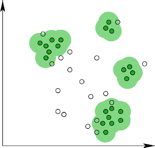
There is a general rule that evaluates the type of clusters being formed by a particular clustering algorithm. The objects (data points) within a particular cluster has to be very similar to the other objects (in that cluster) i.e. the within-cluster homogeneity has to be very high but on the other hand, the objects of a particular cluster have to be as dissimilar as possible to the objects present in other cluster(s).

Although the central idea of clustering (i.e. grouping similar objects together) remains the same, it is important to note that there are various types of clustering which we are going to study in the next section.

Common clustering methods

Based on the way the clusters are formed from the data, there can be different types of clustering methods. We will be studying the most popular types of clustering techniques that are extensively used by organizations. These types are:

Partitioning methods

Partition-based clustering methods cluster the given objects by measuring their distances from either random or some specified objects on an n-dimensional plane. For this reason, these methods are also known as distance-based methods. Euclidean distance, Taxicab distance etc. are generally used for measuring the distances. However, in order to begin the clustering process, partition-based methods require the number of clusters to be formed from the data. Thus, to get the optimal clusters, an exhaustive search space may have to be explored by these methods for large volumes of data. This can indeed be computationally very expensive.

Examples of partition-based clustering methods include K-Means, K-Medoids, CLARANS, etc.

Hierarchical methods

Hierarchical clustering methods are different from the partitioning methods. They split the data points into levels/hierarchies based on their similarities. These levels together form a tree-like structure (called dendrogram). This split can take place in two ways - top-down and bottom-up.

In the top-down (also called divisive) variant, all the data points are considered to be the part of one big cluster and then they get further split into cluster until some stopping criterion is met. On the other hand, the bottom-up or agglomerative method of clustering considers each of the data points as separate clusters and iteratively groups them until a condition(s) is met.

Hierarchical methods fail to perform effectively when it comes to large datasets as there can be a wide array of splitting criteria and the computational cost of exploring each of those criteria can get extensive.

Popular examples of hierarchical clustering methods include BIRCH and Chameleon.

Density-based methods

Instead of considering the distance of the data points, in density-based clustering methods, a neighborhood is considered to form clusters. Neighborhood refers to the number of data points here that are needed to be present around a region of interest (another data point typically) for forming a cluster from the given data. This very idea of several data points surrounding a particular data point gives birth to the notion of density and hence the name. Partitioning methods are good at forming spherically shaped clusters. Density-based methods can handle arbitrary shapes too and this is where lies their advantage.

DBSCAN, OPTICS are the most popular density-based clustering methods.

We now have an overview of the common clustering methods that are applied heavily in the industry. We will now ourselves into a case study in Python where we will take the K-Means clustering algorithm and will dissect its several components.

Dissecting the K-Means algorithm with a case study

In this section, we will unravel the different components of the K-Means clustering algorithm. K-Means is a partition-based method of clustering and is very popular for its simplicity. We will start this section by generating a toy dataset which we will further use to demonstrate the K-Means algorithm. You can follow this Jupyter Notebook to execute the code snippets alongside your reading.

Generating a toy dataset in Python

We will use the make_blobs method module from sklearn.datasets module for doing this. Our dataset would look like the following:

Here’s the code to generate it:

# Imports
from sklearn.datasets.samples_generator import make_blobs

# Generate 2D data points
X, _ = make_blobs(n_samples=10, centers=3, n_features=2,
                 cluster_std=0.2,  random_state=0)

# Convert the data points into a pandas DataFrame
import pandas as pd

# Generate indicators for the data points
obj_names = []
for i in range(1, 11):
    obj = "Object " + str(i)
    obj_names.append(obj)

# Create a pandas DataFrame with the names and (x, y) coordinates
data = pd.DataFrame({
    'Object': obj_names,
    'X_value': X[:, 0],
    'Y_value': X[:, -1]
})

# Preview the data
print(data.head())

Once the above script is successfully run, you should get the following output:

Visually, the dataset looks like so:

We have a total of 10 data points with their x and y coordinates. We will give this data as the input to the K-Means algorithm. From the above scatter plot, it is clear that the data points can be grouped into 3 clusters (but a computer may have a very hard time figuring that out). So, we will ask the K-Means algorithm to cluster the data points into 3 clusters.

K-Means in a series of steps (in Python)

To start using K-Means, you need to specify the number of K which is nothing but the number of clusters you want out of the data. As mentioned just above, we will use K = 3 for now.

Let’s now see the algorithm step-by-step:

• Initialize random centroids

You start the process by taking three(as we decided K to be 3) random points (in the form of (x, y)). These points are called centroids which is just a fancy name for denoting centers. Let’s name these three points - C1, C2, and C3 so that you can refer them later.

• Calculate distances between the centroids and the data points

 Next, you measure the distances of the data points from these three randomly             chosen points. A very popular choice of distance measurement function, in this         case, is the Euclidean distance.

     Briefly, if there are n points on a 2D space(just like the above figure) and their           coordinates are denoted by (x_i, y_i), then the Euclidean distance between any         two points ((x1, y1) and(x2, y2)) on this space is given by:

       Suppose the coordinates of C1, C2 and C3 are - (-1, 4), (-0.2, 1.5) and (2, 2.5)         respectively. Let’s now write a few lines of Python code which will calculate the           Euclidean distances between the data-points and these randomly chosen                     centroids. We start by initializing the centroids.

# Initialize the centroids
c1 = (-1, 4)
c2 = (-0.2, 1.5)
c3 = (2, 2.5)

   Next, we write a small helper function to calculate the Euclidean distances                   between the data points and centroids.

# A helper function to calculate the Euclidean diatance between the data 
# points and the centroids

def calculate_distance(centroid, X, Y):
    distances = []
        
    # Unpack the x and y coordinates of the centroid
    c_x, c_y = centroid
        
    # Iterate over the data points and calculate the distance using the           # given formula
    for x, y in list(zip(X, Y)):
        root_diff_x = (x - c_x) ** 2
        root_diff_y = (y - c_y) ** 2
        distance = np.sqrt(root_diff_x + root_diff_y)
        distances.append(distance)
        
    return distances

 We can now apply this function to the data points and assign the results in the        DataFrame accordingly.

# Calculate the distance and assign them to the DataFrame accordingly
data['C1_Distance'] = calculate_distance(c1, data.X_value, data.Y_value)
data['C2_Distance'] = calculate_distance(c2, data.X_value, data.Y_value)
data['C3_Distance'] = calculate_distance(c3, data.X_value, data.Y_value)

# Preview the data
print(data.head())

   The output should be like the following:

  Time to study the next step in the algorithm.

• Compare, assign, mean and repeat

This is fundamentally the last step of the K-Means clustering algorithm. Once             you have the distances between the data points and the centroids, you compare         the distances and take the smallest ones. The centroid to which the distance for         a particular data point is the smallest, that centroid gets assigned as the cluster         for that particular data point. Let’s do this programmatically.

    # Get the minimum distance centroids
    data['Cluster'] = data[['C1_Distance', 'C2_Distance', 'C3_Distance']].apply(np.argmin, axis =1)
    
    # Map the centroids accordingly and rename them
    data['Cluster'] = data['Cluster'].map({'C1_Distance': 'C1', 'C2_Distance': 'C2', 'C3_Distance': 'C3'})
    
    # Get a preview of the data
    print(data.head(10))

You get a nicely formatted output:

With this step, we complete an iteration of the K-Means cloistering algorithm.            Take a closer look at the output - there’s no C2 in there.

    Now comes the most interesting part of updating the centroids by determining          the mean values of the coordinates of the data points (which should be                        belonging to some centroid by now). Hence the name K-Means. This is how the        mean calculation looks like:

 The following lines of code does this for you:

# Calculate the coordinates of the new centroid from cluster 1
x_new_centroid1 = data[data['Cluster']=='C1']['X_value'].mean()
y_new_centroid1 = data[data['Cluster']=='C1']['Y_value'].mean()

# Calculate the coordinates of the new centroid from cluster 2
x_new_centroid2 = data[data['Cluster']=='C3']['X_value'].mean()
y_new_centroid2 = data[data['Cluster']=='C3']['Y_value'].mean()

# Print the coordinates of the new centroids
print('Centroid 1 ({}, {})'.format(x_new_centroid1, y_new_centroid1))
print('Centroid 2 ({}, {})'.format(x_new_centroid2, y_new_centroid2))

You get:

Notice that the algorithm, in its first iteration, grouped the data points into two     clusters although we specified this number to be 3. The following animation gives     you a pretty good overview of how centroid updates take place in the K-Means           algorithm.

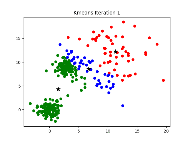
But when does it stop? This process is repeated until the coordinates of the                 centroids do not get updated anymore.

We have now studied the major steps that are involved in the K-Means algorithm. We will now implement this using scikit-learn. In the later sections, We will visualize the clusters formed by the algorithm. We will also study how to evaluate a clustering algorithm. Note that the terms centroids and clusters have been used interchangeably in many cases here.

Making lives easier: K-Means clustering with scikit-learn

The K-Means method from the sklearn.cluster module makes the implementation of K-Means algorithm really easier.

# Using scikit-learn to perform K-Means clustering
from sklearn.cluster import KMeans
    
# Specify the number of clusters (3) and fit the data X
kmeans = KMeans(n_clusters=3, random_state=0).fit(X)

We specified the number of desired clusters to be 3 (the value of K). After that, we gave the data points as the inputs to the K-Means model and trained the model. Let’s now extract the cluster centroids and the cluster labels from the K-Means variable.

# Get the cluster centroids
print(kmeans.cluster_centers_)
    
# Get the cluster labels
print(kmeans.labels_)

It should produce the following output:

But nothing beats visual inspection of the results. Let’s plot the cluster centroids with respect to the data points.

# Plotting the cluster centers and the data points on a 2D plane
plt.scatter(X[:, 0], X[:, -1])
    
plt.scatter(kmeans.cluster_centers_[:, 0], kmeans.cluster_centers_[:, 1], c='red', marker='x')
    
plt.title('Data points and cluster centroids')
plt.show()

You get a plot like:

The above figure is way more informative than the descriptive results shown above. We still have two extremely questions to answer:

• How does one evaluate the performance of a clustering algorithm?
• How to decide the ideal value of K in K-Means?

The questions complement each other. Let’s now find their answers.

Evaluating a clustering algorithm and choosing ‘K’

For this section, the clustering algorithm would be K-Means but the concepts can be applied to any clustering algorithm in general.

An assumption to consider before going for clustering

To apply clustering to a set of data points, it is important to consider that there has to be a non-random structure underlying the data points. To understand this, let’s consider the following data points:

Just by eye-balling at the above data points are you able to see any cluster patterns? To find out clusters from the data, the data should ideally be non-uniformly distributed. Statistical tests like Hopkins Statistic allows you to figure out if the underlying distribution of the data points follow a uniform distribution or not. This might seem easy when you have 2D data points but with an increasing number of dimensions, it gets really difficult.

Cluster evaluation: the silhouette score

When we were preparing our toy dataset, we made sure that the points were not drawn from a uniform distribution (refer the scatter plot in the Generating a toy dataset in Python section, it does not lie).

Now coming to evaluating a clustering algorithm, there are two things to consider here:

• If we have the ground truth labels (class information) of the data points available with us (which is not the case here) then we can make use of extrinsic methods like homogeneity score, completeness score and so on.
• But if we do not have the ground truth labels of the data points, we will have to use the intrinsic methods like silhouette score which is based on the silhouette coefficient. We now study this evaluation metric in a bit more details.
• Let’s start with the equation for calculating the silhouette coefficient for a particular data point:

where,

- s(o) is the silhouette coefficient of the data point o

- a(o) is the average distance between o and all the other data points in the             cluster to which o belongs

   - b(o) is the minimum average distance from o to all clusters to which o does             not belong

The value of the silhouette coefficient is between [-1, 1]. A score of 1 denotes the best meaning that the data point o is very compact within the cluster to which it belongs and far away from the other clusters. The worst value is -1. Values near 0 denote overlapping clusters.

With scikit-learn, you can calculate the silhouette coefficients for all the data points very easily:

# Calculate silhouette_score
from sklearn.metrics import silhouette_score

print(silhouette_score(X, kmeans.labels_))

We get a score of 0.8810668519873335 which is good enough. The                           silhouette_score() function takes two arguments primarily - the data points (X)         and the cluster labels (kmeans.labels_) and returns the mean silhouette                       coefficient of all samples.

   We will now see how to use the silhouette coefficient to determine a good value          for K.

Using silhouette coefficients to determine K: The elbow method

This is a highly iterative process (and an NP-Hard one too) and there is no golden rule of thumb for determining the appropriate value of K (if not by performing a hyperparameters’ search). It largely depends on the kind of data points on which clustering is being applied. However, there is a method known as the elbow method which works pretty well in practice:

• Train a number of K-Means models using different values of K
• Record the average silhouette coefficient during each training
• Plot the silhouette score vs. number of clusters (K) graph
• Select the value of K for which silhouette score is the highest

Let’s implement this in Python now. We will use the yellowbrick library for doing this:

# Import the KElbowVisualizer method 
from yellowbrick.cluster import KElbowVisualizer

# Instantiate a scikit-learn K-Means model
model = KMeans(random_state=0)

# Instantiate the KElbowVisualizer with the number of clusters and the metric 
visualizer = KElbowVisualizer(model, k=(2,6), metric='silhouette', timings=False)

# Fit the data and visualize
visualizer.fit(X)    
visualizer.poof()   

We quickly trained three different K-Means models with 2, 3, 4 and 5 as the values of K. The output of the above code snippet should resemble the following:

We can see that for K = 3, we get the highest average silhouette coefficient. The figure loosely resembles an elbow, hence the name of the method. With this, we can move on to the final section of this article.

Conclusion and further notes

Thank you for making it till the end of this article. We took a whirlwind tour of unsupervised learning in this article including a case study of the good old K-Means algorithm in Python. We implemented many things from scratch but also used the legacy libraries like scikit-learn. In this final section, I wanted to discuss the limitations of K-Means algorithm and wanted to give you some further references to study.

Limitations of K-Means

K-Means is very susceptible to outliers. The algorithm starts by picking up a random set of centroids and iteratively builds its way around. The cluster centroids are updated using the mean values. This is what makes the algorithm prone to outliers.

Consider this set of 1-D data points - {10, 11, 13, 15, 20, 22, 23, 91} and you are asked to cluster them into two groups. It is safe enough to say that 91 is an outlier here and two possible cluster groups would be {10, 11, 13, 15} and {20, 22, 23}.

To give you a sense of the problem that can arise here, let me introduce the concept of within-cluster variation:

Let’s now break down each of the components of the equation:

• k = number of clusters formed
• C_i = centroid of i-th cluster
• p = a data point from the given data
• dist() is the function which produces squared distance between two given points

Now, consider, the K-Means algorithm has formed two clusters - {10, 11, 13, 15} and {20, 22, 23, 91}. The within-cluster variation for this would be:

The centroids of the two clusters were - 12.25 and 44.66.

Now consider another iteration of the algorithm where the partitioning is - {10, 11, 13, 15, 20} and {22, 23, 91}. The within-cluster variation for this will be:

The second partition yielded the lesser within-cluster variation and for this reason, 20 gets assigned to the first cluster. This could have been avoided if we could allow K-Means to treat 91 as an abnormal data point. This very way of calculating the variation using the mean makes K-Means perform very poorly and hence it shows instability in forming the clusters. To prevent this issue, several variants have been proposed such as - K-Medoids, K-Modes.

By now, we have a decent idea of how unsupervised learning a.k.a clustering plays an important role in solving some of the most critical real-world challenges. We also know how the K-Means clustering algorithm works and its nuances. Allow me to give you some references so that you can study more about unsupervised learning in general (if you are interested).

What’s next?

In this article, we barely scratched the surface of the whole world of unsupervised learning. There are other clustering algorithms as well which we did not discuss. But there are always further studies if you want to own something. Following are some of my favorite resources using which can take your knowledge of unsupervised learning to the next level:

• Clustering | KMeans Algorithm, a video lecture by Andrew Ng
• Chapter 10 of  Data Mining. -Concepts and Techniques (3rd Edition) by Han et al. for the other variants of clustering
• Chapter 9 of The Hundred Page Machine Learning Book by Andriy Burkov for density-based estimations in unsupervised learning
• Chapter 9 of Pattern Recognition and Machine Learning by Christopher M. Bishop which discusses the topic of unsupervised learning from a very unique perspective
• Unsupervised Deep Learning (A tutorial presented at NIPS 2018) which shows the usage of deep learning in an unsupervised paradigm
• A robust and sparse K-means clustering algorithm, a paper which discusses many novel approaches for overcoming the limitations of the traditional K-Means algorithm
• Deep Unsupervised Learning, a full-fledged course offered by UC Berkley

That is all for this article. I’d love to hear about your ventures into building your own cool unsupervised learning applications.  

Thanks to Alessio and Bharath of FloydHub for sharing their valuable feedback on the article. Big thanks to the entire FloydHub team for letting me run the accompanying notebook on their platform. If you haven’t checked FloydHub yet, give FloydHub a spin for your Machine Learning and Deep Learning projects. There is no going back once you’ve learned how easy they make it.

FloydHub Call for AI writers

Want to write amazing articles like Sayak and play your role in the long road to Artificial General Intelligence? We are looking for passionate writers, to build the world's best blog for practical applications of groundbreaking A.I. techniques. FloydHub has a large reach within the AI community and with your help, we can inspire the next wave of AI. Apply now and join the crew!

About Sayak Paul

Sayak loves everything deep learning. He goes by the motto of understanding complex things and helping people understand them as easily as possible. Sayak is an extensive blogger and all of his blogs can be found here. He is also working with his friends on the application of deep learning in Phonocardiogram classification. Sayak is also a FloydHub AI Writer. He is always open to discussing novel ideas and taking them forward to implementations. You can connect with Sayak on LinkedIn and Twitter.