Building Your First ConvNet

Convolutional Neural Networks (ConvNets) are increasingly popular, and for all the right reasons. ConvNets have the unique property of retaining translational invariance. In elaborative terms, they exploit spatially-local correlation by enforcing a local connectivity pattern between neurons of adjacent layers.

To learn more about ConvNets or Convolutions in general, you can read about them on Christopher Olah’s blog here –

1. ConvNets: A Modular Perspective
2. Understanding Convolutions

My goal in this post is to help you get up to speed on training ConvNet models in the cloud without the hassles of setting up a VM, AWS instance, or anything of that sort. You’ll be able to design your own classification task with lots of images and train your own ConvNet models.

All you need is some knowledge of Python and the basics of Keras – one of the quintessential deep learning libraries. The data and implementation used here is inspired from this post on the official Keras blog.

Setup

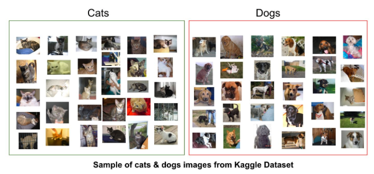
As in any binary classification task, our primary requirement is the data itself - more explicitly, a dataset segregated into 2 classes.

For this purpose, I’m using a simple dataset – DogsVsCats from Kaggle. It is one of the most rudimentary yet popular classifications available - whether an image contains a dog or a cat. For simplicity, I’ve bundled 1,000 images of dogs & cats each and created a project directory with the following structure.

├── train
	├── cats
	├── dogs
└── val
	├── cats
	├── dogs
└── test

The public dataset can be accessed on FloydHub at sominw/datasets/dogsvscats/1.

If you haven’t already setup an account on FloydHub, you can do so by using the FloydHub QuickStart documentation. It’s incredibly simple - you'll be up and running with FloydHub in just a few minutes. If you encounter any issues, the FloydHub forum can provide additional support.

Cloning the Git Repo

I’ve prepared a starter project using our dataset that will allow you to tinker with the model we’re building and help you understand the basics of training models with large datasets on FloydHub. Navigate to a directory of your choice and enter the following:

$ git clone https://github.com/sominwadhwa/DogsVsCats-Floyd.git

Creating a Project on FloydHub

Now it’s time to initialise the project on FloydHub.

1. Create & name your project under your account on FloydHub web dashboard
2. Locally, within your terminal, head over to the project directory and initialize the project with FloydHub

$ floyd init [project-name]

Code

Let's do a quick run-thru of our code: ver_little_data.py.

Prerequisites

from keras.preprocessing.image import ImageDataGenerator, array_to_img, img_to_array, load_img
from keras.models import Sequential
from keras.layers import Conv2D, MaxPooling2D
from keras.layers import Dropout, Activation, Flatten, Dense
from keras.callbacks import ModelCheckpoint, TensorBoard
import h5py
from keras import backend as K
import numpy as np

• NumPy: NumPy is a scientific computing package in Python. In context of Machine Learning, it is primarily used to manipulate N-Dimensional Arrays & some linear algebra and random number capabilities. (Documentation)

• Keras: Keras is a high level neural networks API used for rapid prototyping. We’ll be running it on top of TensorFlow, an open source library for numerical computation using data flow graphs. (Documentation)

• h5py: Used simultaneously with NumPy to store huge amounts of numerical data in HDF5 binary data format. (Documentation)

• Tensorboard: Tool used to visualize the static compute graph created by TensordFlow, plot quantitative metrics during the execution, and show additional information about it. (Concise Tutorial)

width, height = 150, 150
training_path = "/input/train"
val_path = "/input/val"
n_train = 2000
n_val = 400
epochs = 100
batch_size = 32

The above snippet defines the training & validation paths. /input is the default mount point of any directory (root) uploaded as data on Floyd. The dataset used here is a publically accessible, so you'll be able to connect it with your own project on FloydHub.

Model Architecture

model = Sequential()
model.add(Conv2D(32,(3,3), input_shape= input_shape))
model.add(Activation('relu'))
model.add(MaxPooling2D(pool_size=(2,2)))

model.add(Conv2D(32,(3,3)))
model.add(Activation('relu'))
model.add(MaxPooling2D(pool_size=(2,2)))

model.add(Conv2D(64, (3,3)))
model.add(Activation('relu'))
model.add(MaxPooling2D(pool_size=(2,2)))

model.add(Flatten())
model.add(Dense(64))
model.add(Activation('relu'))
model.add(Dropout(0.4))
model.add(Dense(1))
model.add(Activation('sigmoid'))

model.compile(loss='binary_crossentropy',
        optimizer='rmsprop',
        metrics=['accuracy'])

Keras makes it incredibly simple to sequentially stack fully configurable modules of neural layers, cost functions, optimizers, activation functions, and regularization schemes over one another.

For this demonstration, we’ve stacked three 2D ConvNet layers (1 Input, 2 Hidden) with ReLu activation. To control overfitting, there’s a 40% dropout before the final activation in the last layer of the network along with MaxPooling layers. For the loss function, since this is a standard binary classification problem, binary_crossentropy is a standard choice. To read and learn more about Cross-Entropy loss, you can checkout this article by Rob DiPietro.

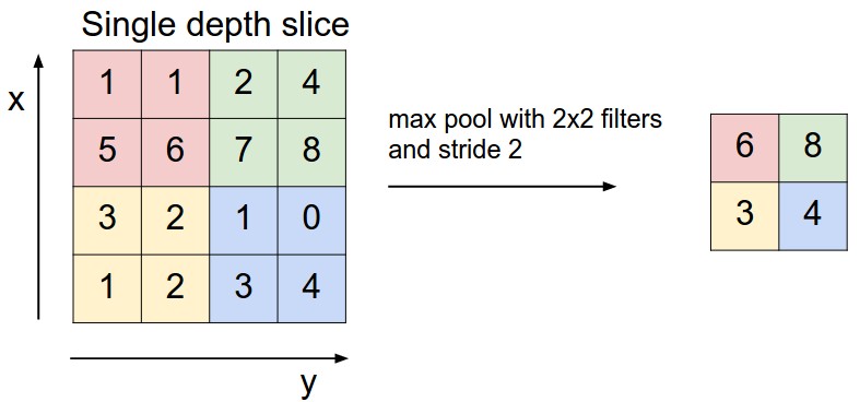
Pooling: One indispensable part of a ConvNet is the Pooling Layer. It serves two primary purposes. By progressively reducing the spatial size of the representation, it retains ‘translational invariance’ in the network and by virtue of that it also reduces the amount of parameters and computation in the network, hence also controlling overfitting. Pooling is often applied with filters of size 2x2 with a stride of 2 at every depth slice. A pooling layer of size 2x2 with stride of 2 shrinks the input image to 1/4 of its original size.

Data Preparation

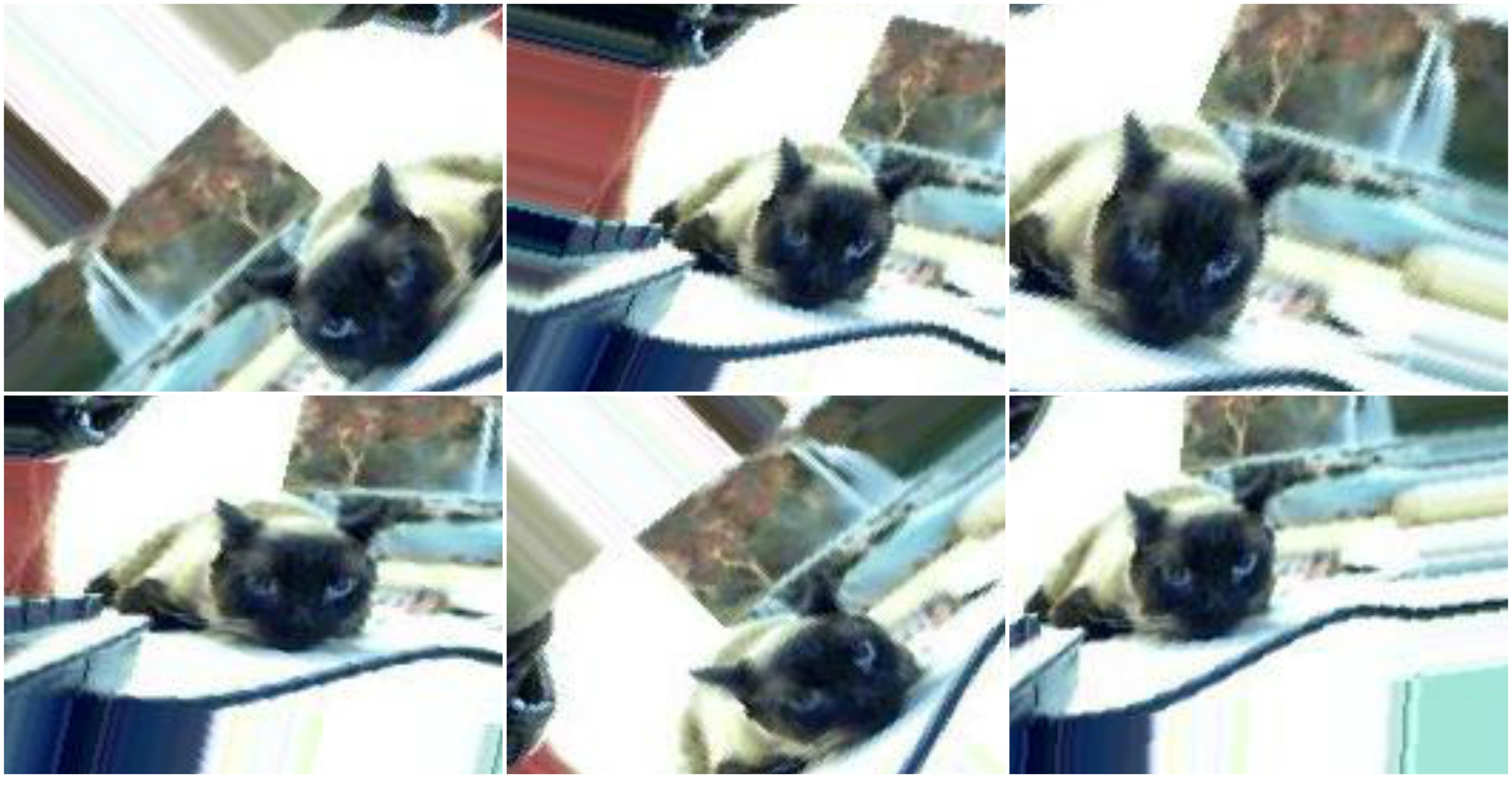
Since we’re using very little data (1k training examples per class), we try to augment these examples by a number of different image transformations using ImageGenerator class in Keras.

train_data = ImageDataGenerator(
        rescale= 1./255,
        shear_range=0.2,
        zoom_range=0.2,
        horizontal_flip=True)

train = train_data.flow_from_directory(
        training_path,
        class_mode='binary',
        batch_size=batch_size,
        target_size=(width,height))

So with a single image, we can generate a lot more belonging to the same class, containing the same object but in a slightly different form.

Tensorboard

Tensorboard is a visualization tool provided with TensorFlow that allows us to visualize TensorFlow compute graphs among other things.

tensorboard = TensorBoard(log_dir='/output/Graph', histogram_freq=0, write_graph=True, write_images=True)

Keras provides callbacks to implement Tensorboard among other procedures to keep a check on the internal states and statistics of the model during training.

FloydHub provides support for TensorBoard inclusion in your jobs. For instance, the above snippet stores the TensorBoard logs in a directory /output/Graph and generates the graph in real time.

Training

So now that we’ve thoroughly dissected the code, it’s finally time to train this network on the cloud. To run this job on FloydHub, simply run the following in your terminal (after navigating to the project directory):

$ floyd run --data sominw/datasets/dogsvscats/1:input --gpu --tensorboard "python very_little_data.py --logdir /output/Graph"

• --logdir flag provides a directory for storing the tensorboard logs.
• --gpu (optional) indicates that you wish to use the GPU compute.
• --tensorboard indicates the usage of Tensorboard.

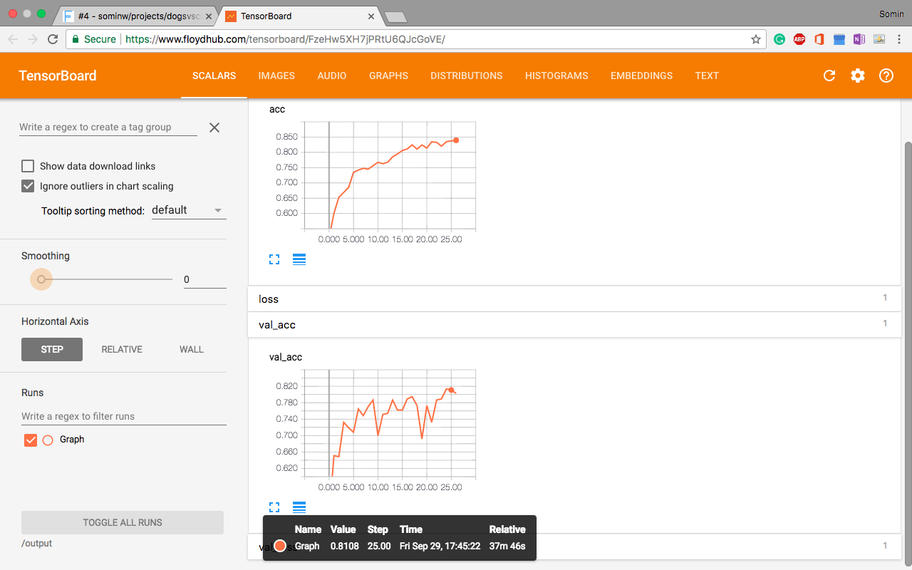
Upon indicating that you’re using Tensorboard (while executing the job), FloydHub provides a direct link to access the Tensorboard. You can read more about Tensorboard support on FloydHub on Naren's post.

Outputs

Keras lets you store multi dimensional numerical matrices in the form of weights in HDF5 Binary data format.

model.save_weights('/output/very_little_weights.hdf5')

The snippet above stores your generated weight file, at the end of training, to the /output directory. You can view the output of your job on FloydHub's dashboard using the Output tab.

And that’s it! You’ve finally trained and visualized your first scalable ConvNet.

I’ll encourage you to try out your own variants of ConvNets by editing the source code. In fact, you can refer to this article and build an even more powerful ConvNet by using pre-trained VGG weights.

If you’d like to read more about running instances on FloydHub, including how to use Datasets and running jobs with external dependencies, you can read my previous article on FloydHub’s blog: Getting Started with Deep Learning on FloydHub.

References

• Building powerful image classification models using very little data - Keras Official Blog
• ConvNets: A modular approach
• Emil Walner: My first weekend of Deep Learning
• Intro to Cross Entropy Loss

About Somin Wadhwa

Somin is currently majoring in Computer Science & is a research intern at Complex Systems Lab, IIIT-Delhi. His areas of interest include Machine Learning, Statistical Data Analysis & Basketball.

You can follow along with him on Twitter or LinkedIn.

We're always looking for more guests to write interesting blog posts about deep learning. Let us know on Twitter if you're interested.