Have you ever trained a pet and rewarded it for every correct command you asked for? Do you know that this simple way of rewarding behavior can be modeled in a robot or a software program to make it do useful things? In this article, we are going to step into the world of reinforcement learning, another beautiful branch of artificial intelligence, which lets machines learn on their own in a way different from traditional machine learning. Particularly, we will be covering the simplest reinforcement learning algorithm i.e. the Q-Learning algorithm in great detail.

In the first half of the article, we will be discussing reinforcement learning in general with examples where reinforcement learning is not just desired but also required. We will then study the Q-Learning algorithm along with an implementation in Python using Numpy.

Let’s start, shall we?

The brass tacks: What is reinforcement learning?

Throughout our lives, we perform a number of actions to pursue our dreams. Some of them bring us good rewards and others do not. Along the way, we keep exploring different paths and try to figure out which action might lead to better rewards. We work hard towards our dreams utilizing the feedback we get based on our actions to improve our strategies. They help us determine how close we are to achieving our goals. Our mental states change continuously to representing this closeness.

In that description of how we pursue our goals in daily life, we framed for ourselves a representative analogy of reinforcement learning. Let me summarize the above example reformatting the main points of interest.

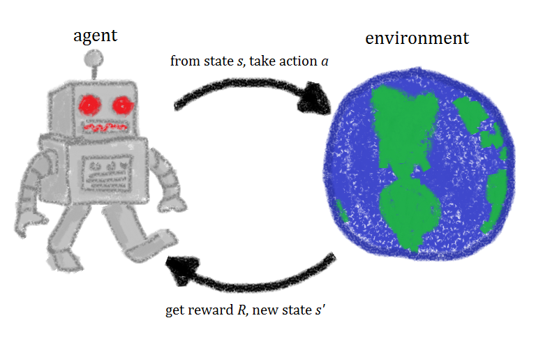
Our reality contains environments in which we perform numerous actions. Sometimes we get good or positive rewards for some of these actions in order to achieve goals. During the entire course of life, our mental and physical states evolve. We strengthen our actions in order to get as many rewards as possible.

The key entities of interest are - environment, action, reward and state. Let’s give ourselves a name as well - we are agents in this whole game of life. This whole paradigm of exploring our lives and learning from it through actions, rewards and states establishes the foundation of reinforcement learning. In fact, this is almost how we act in any given circumstance in our lives, isn’t it?

It turns out that the whole idea of reinforcement learning is pretty empirical in nature. Now, think for a moment, how would we train robots and machines to do the kind of useful tasks we humans do. Be it switching off the television, or moving things around, or organizing bookshelves. Fundamentally, these tasks are not about finding a function mapping inputs to outputs or finding hidden representations within input data. These are a completely different set of tasks and require a different learning paradigm for a computer to be able to perform these tasks. Andriy Burkov in his The Hundred Page Machine Learning Book describes reinforcement learning as:

Reinforcement learning solves a particular kind of problem where decision making is sequential, and the goal is long-term, such as game playing, robotics, resource management, or logistics.

For a robot, an environment is a place where it has been put to use. Remember this robot is itself the agent. For example, a textile factory where a robot is used to move materials from one place to another. We will come to its states, actions, rewards later. The tasks we discussed just now, have a property in common -  these tasks involve an environment and expect the agents to learn from that environment. This is where traditional machine learning fails and hence the need for reinforcement learning.

So, the headline AI Bots Join Forces To Beat Top Human Dota 2 Team that shook the gaming world is a direct byproduct of reinforcement learning. Beyond beating humans in game-playing, there are some other marvelous use cases of reinforcement learning:

• Optimizing business processes
• Minimizing energy costs
• Maximizing revenue shares of a company

and lots more.

In the next section, we will begin by defining the problem which is very relevant in the field of reinforcement learning. After that, we will study its agents, environment, states, actions and rewards. We will then directly proceed towards the Q-Learning algorithm.

Recipes for reinforcement learning

It is good to have an established overview of the problem that is to be solved using reinforcement learning, Q-Learning in this case. It helps to define the main components of a reinforcement learning solution i.e. agents, environment, actions, rewards and states.

Defining the problem statement

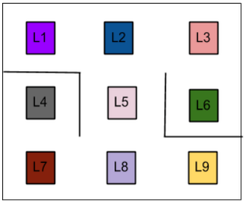
We are to build a few autonomous robots for a guitar building factory. These robots will help the guitar luthiers by conveying them the necessary guitar parts that they would need in order to craft a guitar. These different parts are located at nine different positions within the factory warehouse. Guitars parts include polished wood stick for the fretboard, polished wood for the guitar body, guitar pickups and so on. The luthiers have prioritized the location that contains body woods to be the topmost. They have provided the priorities for other locations as well which we will look in a moment. These locations within the factory warehouse look like -

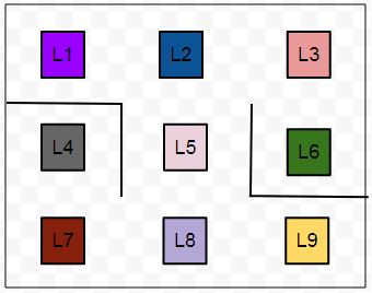
As we can see there are little obstacles present (represented with smoothed lines) in between the locations. L6 is the top-priority location that contains the polished wood for preparing guitar bodies. Now, the task is to enable the robots so that they can find the shortest route from any given location to another location on their own.

The agents, in this case, are the robots. The environment is the guitar factory warehouse.

The states

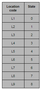
The states are the locations. The location in which a particular robot is present in the particular instance of time will denote its state. Machines understand numbers rather than letters. So, let’s map the location codes to numbers.

The actions

In our example, the actions will be the direct locations that a robot can go to from a particular location. Consider, a robot is at the L8 location and the direct locations to which it can move are L5, L7 and L9. The below figure may come in handy in order to visualize this.

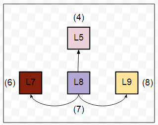
As you might have already guessed the set of actions here is nothing but the set of all possible states of the robot. For each location, the set of actions that a robot can take will be different. For example, the set of actions will change if the robot is in L1.

The rewards

By now, we have the following two sets:

• A set of states: $$S = {0, 1, 2, 3, 4, 5, 6, 7, 8}$$
• A set of actions: $$A = {0, 1, 2, 3, 4, 5, 6, 7, 8}$$

The rewards, now, will be given to a robot if a location (read it state) is directly reachable from a particular location. Let’s take an example:

L9 is directly reachable from L8. So, if a robot goes from L8 to L9 and vice-versa, it will be rewarded by 1. If a location is not directly reachable from a particular location, we do not give any reward (a reward of 0). Yes, the reward is just a number here and nothing else. It enables the robots to make sense of their movements helping them in deciding what locations are directly reachable and what are not. With this cue, we can construct a reward table which contains all the reward values mapping between all the possible states (locations).

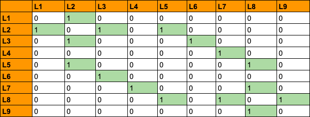
In the above table, we have all the possible rewards that a robot can get by moving in between the different states.

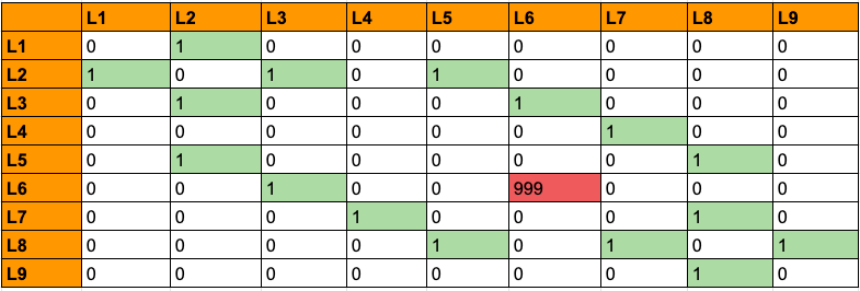
Now comes an interesting decision. Remember from the previous sections that the luthier prioritized L6 to be of the topmost? So, how do we incorporate this fact in the above table? This is done by associating the topmost priority location with a very higher reward than the usual ones. Let’s put 999 in the cell (L6, L6):

We have now formally defined all the vital components for the solution we are aiming for the problem discussed above. We will shift gears a bit and study some of the fundamental concepts that prevail in the world of reinforcement learning. We will start with the Bellman Equation.

The Bellman Equation

Consider the following square of rooms which is analogous to the actual environment from our original problem but without the barriers.

Now suppose a robot needs to go to the room, marked in green from its current position (A) using the specified direction.

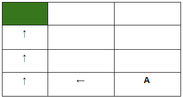
How can we enable the robot to do this programmatically? One idea would be to introduce some kind of footprint which the robot would be able to follow like below.

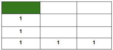
Here, a constant value is specified in each of the rooms which will come along the robot’s way if it follows the direction specified above. In this way, if it starts at location A, it will be able to scan through this constant value and will move accordingly. But this would only work if the direction is prefixed and the robot always starts at location A. Now, consider the robot starts at the following location:

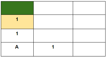
The robot now sees footprints in two different directions. It is, therefore, unable to decide which way to go in order to get to the destination (green room). It happens primarily because the robot does not have a way to remember the directions to proceed. So, our job now is to enable the robot with a memory. This is where the Bellman Equation comes into play:

$$V(s)=\max _{a}\left(R(s, a) + \gamma V\left(s^{\prime}\right)\right)$$

where,

• s = a particular state (room)
• a = action (moving between the rooms)
• s′ = state to which the robot goes from s
• 𝜸 = discount factor (we will get to it in a moment)
• R(s, a) = a reward function which takes a state s and action a and outputs a reward value
• V(s) = value of being in a particular state (the footprint)

We consider all the possible actions and take the one that yields the maximum value.

There is one constraint however regarding the value footprint i.e. the room, marked in yellow just below the green room will always have a value of 1 to denote that it is one of the nearest room adjacent to the green room. This is also to ensure that a robot gets a reward when it goes from the yellow room to the green room. Let’s now see how to make sense of the above equation here.

We will assume a discount factor of 0.9.

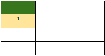
* For this room (read state) what will be V(s)? Let’s put the values into the equation straightly:

$$V(s)=\max _{a}(0 + 0.9 * 1)=0.9$$

Here, the robot will not get any reward for going to the state (room) marked in yellow, hence R(s, a) = 0 here. The robot knows the values of being in the yellow room hence V(s′) is 1. Following this for the other states, we should get:

A couple of things to notice here:

• The max() function helps the robot to always choose the state that gives it the maximum value of being in that state.
• The discount factor 𝜸 notifies the robot about how far it is from the destination. This typically specified by the developer of the algorithm that would be instilled in the robot.

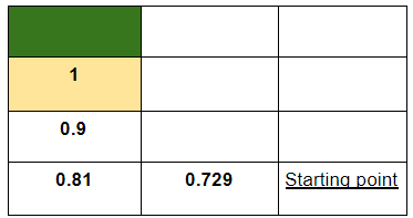
The other states can also be given their respective values in a similar way:

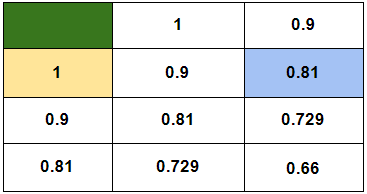
The robot now can proceed its way through the green room utilizing these value footprints even if it is dropped at any arbitrary room in the above square. Now, if a robot lands up in the highlighted (sky blue) room, it will still find two options to choose from. But eventually, either of the paths will be good enough for the robot to take because of the way the value footprints are now laid out.

Notice how the main task of reaching a destination from a particular source got broken down to similar subtasks. It turns out that there is a particular programming paradigm developed especially for solving problems that have repetitive subproblems in them. It is referred to as dynamic programming. It was invented by Richard Bellman in 1954 who also coined the equation we just studied (hence the name, Bellman Equation). Note that this is one of the key equations in the world of reinforcement learning.

If we think realistically, our surroundings do not always work in the way we expect. There is always a bit of stochasticity involved in it. This applies to a robot as well. Sometimes, it might so happen that the robot’s inner machinery got corrupted. Sometimes, the robot may come across some hindrances on its way which may not be known to it beforehand. Sometimes, even if the robot knows that it needs to take the right turn, it will not. So, how do we introduce this stochasticity in our case? Markov Decision Processes.

Modeling stochasticity: Markov Decision Processes

Consider the robot is currently in the red room and it needs to go to the green room.

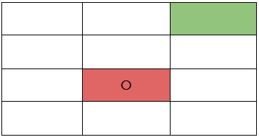
Let’s now consider, the robot has a slight chance of dysfunctioning and might take the left or right or bottom turn instead of taking the upper turn in order to get to the green room from where it is now (red room). Now, the question is how do we enable the robot to handle this when it is out there in the above environment?

This is a situation where the decision making regarding which turn is to be taken is partly random and partly under the control of the robot. Partly random because we are not sure when exactly the robot might dysfunction and partly under the control of the robot because it is still making a decision of taking a turn on its own and with the help of the program embedded into it. Here is the definition of Markov Decision Processes (collected from Wikipedia):

A Markov decision process (MDP) is a discrete time stochastic control process. It provides a mathematical framework for modeling decision making in situations where outcomes are partly random and partly under the control of a decision maker.

You may focus only on the highlighted part. We have the exact same situation here in our case.

We have now introduced ourselves with the concept of partly random and partly controlled decision making. We need to give this concept a mathematical shape (most likely an equation) which then can be taken further.  You might be surprised to see that we can do this with the help of the Bellman Equation with a few minor tweaks.

Here is the original Bellman Equation, again:

$$V(s)=\max _{a}\left(R(s, a) + \gamma V\left(s^{\prime}\right)\right)$$

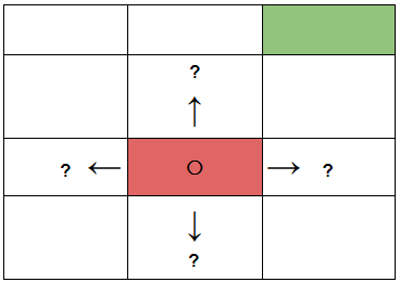
What needs to be changed in the above equation so that we can introduce some amount of randomness here? As long as we are not sure when the robot might not take the expected turn, we are then also not sure in which room it might end up in which is nothing but the room it moves from its current room. At this point, according to the above equation, we are not sure of s′ which is the next state (room, as we were referring them). But we do know all the probable turns the robot might take! In order to incorporate each of these probabilities into the above equation, we need to associate a probability with each of the turns to quantify that the robot has got x% chance of taking this turn. If we do so, we get:

$$V(s)=\max _{a}\left(R(s, a) + \gamma \sum{s^{\prime}} P\left(s, a, s^{\prime}\right) V\left(s^{\prime}\right)\right)$$

Taking the new notations step by step:

• P(s, a, s′) - the probability of moving from room s to room s′ with action a
• $$\sum_{s^{\prime}} P\left(s, a, s^{\prime}\right) V\left(s^{\prime}\right)$$ - expectation of the situation that the robot incurs randomness

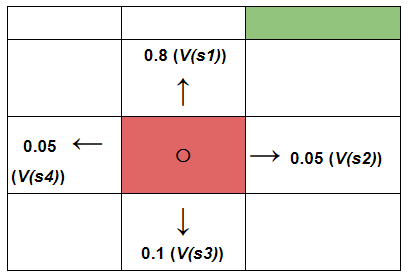
Notice, everything else from the above two points is exactly the same. Let’s assume the following probabilities are associated with each of the turns the robot might take while being in that red room (to go to the green room).

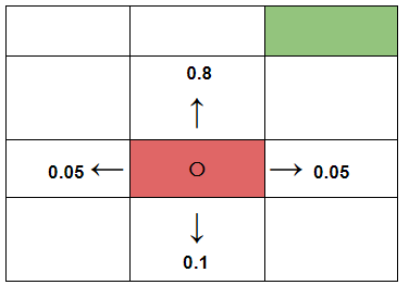
When we associate probabilities to each of these turns, we essentially mean that there is an 80% chance that the robot will take the upper turn. If we put all the required values in our equation, we get:

$$V(s)=\max _{a} (R(s, a) + \gamma((0.8V(room_{up})) +( 0.1V(room_{down})) + ...))$$

Note that the value footprints will now change due to the fact that we are incorporating stochasticity here. But this time, we will not calculate those value footprints. Instead, we will let the robot to figure it out (more on this in a moment).

Up until this point, we have not considered about rewarding the robot for its action of going into a particular room. We are only rewarding the robot when it gets to the destination. Ideally, there should be a reward for every action the robot takes to help it better assess the quality of its actions. The rewards need not be always the same. But it is much better than having some amount reward for the actions than having no rewards at all. This idea is known as the living penalty. In reality, the rewarding system can be very complex and particularly modeling sparse rewards is an active area of research in the domain reinforcement learning. If you would like to give a spin to this topic then following resources might come in handy:

• Curiosity-driven Exploration by Self-supervised Prediction
• Curiosity and Procrastination in Reinforcement Learning
• Learning to Generalize from Sparse and Underspecified Rewards

In the next section, we will introduce the notion of the quality of an action rather than looking at the value of going into a particular room (V(s)).

Transitioning to Q-Learning

By now, we have got the following equation which gives us a value of going to a particular state (form now on, we will refer to the rooms as states) taking the stochasticity of the environment into the account:

$$V(s)=\max {a}\left(R(s, a)  + \gamma \sum{s^{\prime}} P\left(s, a, s^{\prime}\right) V\left(s^{\prime}\right)\right)$$

We have also learned very briefly about the idea of living penalty which deals with associating each move of the robot with a reward.

Q-Learning poses an idea of assessing the quality of an action that is taken to move to a state rather than determining the possible value of the state (value footprint) being moved to.

Earlier, we had:

If we incorporate the idea of assessing the quality of actions for moving to a certain state s′.

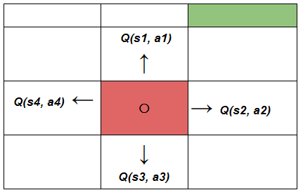
The robot now has four different states to choose from and along with that, there are four different actions also for the current state it is in. So how do we calculate Q(s, a) i.e. the cumulative quality of the possible actions the robot might take? Let’s break down.

From this equation $$V(s)=\max {a}\left(R(s, a) +  \gamma \sum{s^{\prime}} P\left(s, a, s^{\prime}\right) V\left(s^{\prime}\right)\right)$$, if we discard the max() function, we get:

$$R(s, a) + \gamma \sum_{s^{\prime}}\left(P\left(s, a, s^{\prime}\right) V\left(s^{\prime}\right)\right)$$

Essentially, in the equation that produces V(s), we are considering all possible actions and all possible states (from the current state the robot is in) and then we are taking the maximum value caused by taking a certain action. The above equation produces a value footprint is for just one possible action. In fact, we can think of it as the quality of the action:

$$Q(s, a)=R(s, a) + \gamma \sum_{s^{\prime}}\left(P\left(s, a, s^{\prime}\right) V\left(s^{\prime}\right)\right)$$

Now that we have got an equation to quantify the quality of a particular action we are going to make a little adjustment in the above equation. We can now say that V(s) is the maximum of all the possible values of Q(s, a). Let’s utilize this fact and replace V(s′) as a function of Q():

$$Q(s, a)=R(s, a) + \gamma \sum_{s^{\prime}}\left(P\left(s, a, s^{\prime}\right) \max _{a^{\prime}} Q\left(s^{\prime}, a^{\prime}\right)\right)$$

But why would we do that?

To ease our calculations. Because now, we have only one function Q() (which is also at the core of the dynamic programming paradigm) to calculate and R(s, a) is a quantified metric which produces rewards of moving to a certain state. The qualities of the actions are called Q-values. And from now on, we will refer the value footprints as the Q-values.

We now have the last piece of the puzzle remaining i.e. temporal difference before we jump to the implementation part and we are going to study that in the next section.

The last piece of the puzzle: Temporal difference

Recollect the statement from a previous section:

But this time, we will not calculate those value footprints. Instead, we will let the robot to figure it out (more on this in a moment).

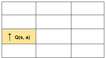
Temporal Difference is the component that will help the robot to calculate the Q-values with respect to the changes in the environment over time. Consider our robot is currently in the marked state and it wants to move to the upper state. Note that the robot already knows the Q-value of making the action i.e. moving to the upper state.  

We know that the environment is stochastic in nature and the reward that the robot will get after moving to the upper state might be different from an earlier observation. So how do we capture this change (read difference)? We recalculate the new Q(s, a) with the same formula and subtract the previously known Q(s, a) from it.

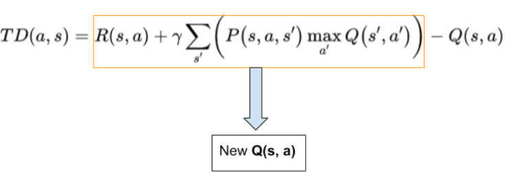
The equation that we just derived gives the temporal difference in the Q-values which further helps to capture the random changes that the environment may impose. The new Q(s, a) is updated as the following:

$$Q_{t}(s, a)=Q_{t-1}(s, a)+\alpha T D_{t}(a, s)$$

where,

• ɑ is the learning rate which controls how quickly the robot adopts to the random changes imposed by the environment
• $$Q_t (s, a)$$ is the current Q-value
• $$Q_{t-1} (s, a)$$ is the previously recorded Q-value

If we replace $$TD_t(s, a)$$ with its full-form equation, we should get:

$$Q_{t}(s, a)=Q_{t-1}(s, a)+\alpha\left(R(s, a)+\gamma \max _{a^{\prime}} Q\left(s^{\prime}, a^{\prime}\right)-Q_{t-1}(s, a)\right)$$

We now have all the little pieces of Q-Learning together to move forward to its implementation part. Feel free to review the problem statement once which we discussed in the very beginning.

Implementing Q-Learning in Python with Numpy

If you do not have a local setup, you can run this notebook directly on FloydHub by just clicking on the below button -

To implement the algorithm, we need to understand the warehouse locations and how that can be mapped to different states. Let’s start by recollecting the sample environment shown earlier:

Let’s map each of the above locations in the warehouse to numbers (states). It will ease our calculations.

# Define the states
location_to_state = {
    'L1' : 0,
    'L2' : 1,
    'L3' : 2,
    'L4' : 3,
    'L5' : 4,
    'L6' : 5,
    'L7' : 6,
    'L8' : 7,
    'L9' : 8
}

We will only be using Numpy as our dependency. So let’s import that aliased as np:

import numpy as np

The next step is to define the actions which as mentioned above represents the transition to the next state:

# Define the actions
actions = [0,1,2,3,4,5,6,7,8]

Now the reward table:

# Define the rewards
rewards = np.array([[0,1,0,0,0,0,0,0,0],
              [1,0,1,0,1,0,0,0,0],
              [0,1,0,0,0,1,0,0,0],
              [0,0,0,0,0,0,1,0,0],
              [0,1,0,0,0,0,0,1,0],
              [0,0,1,0,0,0,0,0,0],
              [0,0,0,1,0,0,0,1,0],
              [0,0,0,0,1,0,1,0,1],
              [0,0,0,0,0,0,0,1,0]])

If you understood it correctly, there isn't any real barrier limitation as depicted in the image. For example, the transition L4 to L1 is allowed but the reward will be zero to discourage that path.

In the above code snippet, we took each of the states and put ones in the respective state that are directly reachable from a certain state. Refer to the reward table once again. The above array construction will be easy to understand then. Note that, we did not consider the top-priority location (L6) yet.

We would also need an inverse mapping from the states back to original location indicators. It will be clearer when we reach to the utter depths of the algorithm. The following line of code will do this for us.

# Maps indices to locations
state_to_location = dict((state,location) for location,state in location_to_state.items())

Before we write a helper function which will yield the optimal route for going from one location to another, let’s specify the two parameters of the Q-Learning algorithm - ɑ (learning rate) and 𝜸 (discount factor).

# Initialize parameters
gamma = 0.75 # Discount factor 
alpha = 0.9 # Learning rate 

We will now define a function get_optimal_route() which will:

• Take two arguments:
• starting location in the warehouse and
• end location in the warehouse respectively
• And will return the optimal route for reaching the end location from the starting location in the form of an ordered list containing the letters

We will start defining the function by initializing the Q-values to be all zeros.

# Initializing Q-Values
Q = np.array(np.zeros([9,9]))

For convenience, we will copy the rewards matrix rewards to a separate variable and will operate on that.

# Copy the rewards matrix to new Matrix
rewards_copy = np.copy(rewards)

[9,9] as we have a total of 9 locations. The function will take a starting location and an ending location. So, let’s set the priority of the ending location to a larger integer like 999 and get the ending state from the location letter (such as L1, L2 and so on).

# Get the ending state corresponding to the ending location as given
ending_state = location_to_state[end_location]

# With the above information automatically set the priority of the
# given ending state to the highest one
rewards_copy[ending_state,ending_state] = 999

Learning is a continuous process, hence we will let the robot to explore the environment for a while and we will do it by simply looping it through 1000 times. We will then pick a state randomly from the set of states we defined above and we will call it current_state.

for i in range(1000):
    # Pick up a state randomly
    current_state = np.random.randint(0,9)

We then, being inside the loop, iterate through the rewards matrix to get the states that are directly reachable from the randomly chosen current state and we will assign those state in a list named playable_actions.

Note that so far we have not bothered about the starting location yet.

playable_actions = []
# Iterate through the new rewards matrix and get the actions > 0
for j in range(9):
    if rewards_copy[current_state,j] > 0:
        playable_actions.append(j)

We will now choose a state randomly from the playable_actions.

# Pick an action randomly from the list of playable actions leading us to the next 
# state
    next_state = np.random.choice(playable_actions)

We can now compute the temporal difference and update the Q-values accordingly. Here is the formula of temporal difference for your convenience:

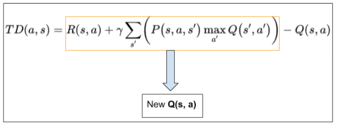
Here is the way to update the Q-values using the temporal difference:

$$Q_{t}(s, a)=Q_{t-1}(s, a)+\alpha T D_{t}(a, s)$$

# Compute the temporal difference
# The action here exactly refers to going to the next state
TD = rewards_copy[current_state,next_state] + gamma * Q[next_state, np.argmax(Q[next_state,])] - Q[current_state,next_state]

# Update the Q-Value using the Bellman equation
Q[current_state,next_state] += alpha * TD

The good news is we are done implementing the most critical part of the process and up until now the definition of get_optimal_route() should look like:

def get_optimal_route(start_location,end_location):
    # Copy the rewards matrix to new Matrix
    rewards_new = np.copy(rewards)
    
    # Get the ending state corresponding to the ending location as given
    ending_state = location_to_state[end_location]
    
    # With the above information automatically set the priority of the given ending 
    # state to the highest one
    rewards_new[ending_state,ending_state] = 999

    # -----------Q-Learning algorithm-----------
   
    # Initializing Q-Values
    Q = np.array(np.zeros([9,9]))

    # Q-Learning process
    for i in range(1000):
        # Pick up a state randomly
        current_state = np.random.randint(0,9) # Python excludes the upper bound
        # For traversing through the neighbor locations in the maze
        playable_actions = []
        # Iterate through the new rewards matrix and get the actions > 0
        for j in range(9):
            if rewards_new[current_state,j] > 0:
                playable_actions.append(j)
        # Pick an action randomly from the list of playable actions  
        # leading us to the next state
        next_state = np.random.choice(playable_actions)
        # Compute the temporal difference
        # The action here exactly refers to going to the next state
        TD = rewards_new[current_state,next_state] + gamma * Q[next_state,                                np.argmax(Q[next_state,])] - Q[current_state,next_state]
        # Update the Q-Value using the Bellman equation
        Q[current_state,next_state] += alpha * TD

We will now start the other half of finding the optimal route. We will first initialize the optimal route with the starting location.

# Initialize the optimal route with the starting location
    route = [start_location]

We currently do not know about the next move of the robot. Thus we will set the next location to also be the starting location.

next_location = start_location

Since we do not know the exact number of iterations the robot will take in order to find out the optimal route, we will simply loop the next set of processes until the next location is not equal to the ending location. This is where we will terminate the loop.

# We don't know about the exact number of iterations needed to reach to the final 
# location hence while loop will be a good choice for iteratiing
    while(next_location != end_location):
        # Fetch the starting state
        starting_state = location_to_state[start_location]
        # Fetch the highest Q-value pertaining to starting state
        next_state = np.argmax(Q[starting_state,])
        # We got the index of the next state. But we need the corresponding letter. 
        next_location = state_to_location[next_state]
        route.append(next_location)
        # Update the starting location for the next iteration
        start_location = next_location
    
    return route

Finally, we return the route.

return route

Here is the whole get_optimal_route() function:

def get_optimal_route(start_location,end_location):
    # Copy the rewards matrix to new Matrix
    rewards_new = np.copy(rewards)
    
    # Get the ending state corresponding to the ending location as given
    ending_state = location_to_state[end_location]
    
    # With the above information automatically set the priority of  
    # the given ending state to the highest one
    rewards_new[ending_state,ending_state] = 999

    # -----------Q-Learning algorithm-----------
   
    # Initializing Q-Values
    Q = np.array(np.zeros([9,9]))

    # Q-Learning process
    for i in range(1000):
        # Pick up a state randomly
        current_state = np.random.randint(0,9) # Python excludes the upper bound
        
        # For traversing through the neighbor locations in the maze
        playable_actions = []
        
        # Iterate through the new rewards matrix and get the actions > 0
        for j in range(9):
            if rewards_new[current_state,j] > 0:
                playable_actions.append(j)
        
        # Pick an action randomly from the list of playable actions  
        # leading us to the next state
        next_state = np.random.choice(playable_actions)
        
        # Compute the temporal difference
        # The action here exactly refers to going to the next state
        TD = rewards_new[current_state,next_state] + gamma * Q[next_state,                         np.argmax(Q[next_state,])] - Q[current_state,next_state]
        
        # Update the Q-Value using the Bellman equation
        Q[current_state,next_state] += alpha * TD

    # Initialize the optimal route with the starting location
    route = [start_location]
    # We do not know about the next location yet, so initialize with the value of 
    # starting location
    next_location = start_location
    
    # We don't know about the exact number of iterations
    # needed to reach to the final location hence while loop will be a good choice 
    # for iteratiing
    
    while(next_location != end_location):
        # Fetch the starting state
        starting_state = location_to_state[start_location]
        
        # Fetch the highest Q-value pertaining to starting state
        next_state = np.argmax(Q[starting_state,])
        
        # We got the index of the next state. But we need the corresponding letter. 
        next_location = state_to_location[next_state]
        route.append(next_location)
        
        # Update the starting location for the next iteration
        start_location = next_location
    
    return route

If we call print(get_optimal_route('L9', 'L1')), we should get:

['L9', 'L8', 'L5', 'L2', 'L1']

Note how the program considers the barriers that are present in the environment. For fun, you can change the ɑ and 𝜸 parameters to see how the learning process changes. With this, let me move to the conclusion section where we will be discussing how you can take your reinforcement learning journey further.

Let’s refactor the code a little bit to conform to OOP paradigm. We will define a class named QAgent() containing the following two methods apart from init:

• training(self, start_location, end_location, iterations) which will help the robot to obtain the Q-values from the environment
• get_optimal_route(self, start_location, end_location, next_location, route, Q) which will get the robot an optimal route from a point to another

Let’s first define the __init__() method which would initialize the class constructor:

def __init__(self, alpha, gamma, location_to_state, actions, rewards, state_to_location, Q):
        
    self.gamma = gamma  
    self.alpha = alpha 

    self.location_to_state = location_to_state
    self.actions = actions
    self.rewards = rewards
    self.state_to_location = state_to_location

    self.Q = Q

Now comes the training() method:

def training(self, start_location, end_location, iterations):

    rewards_new = np.copy(self.rewards)

    ending_state = self.location_to_state[end_location]
    rewards_new[ending_state, ending_state] = 999

    for i in range(iterations):
        current_state = np.random.randint(0,9) 
        playable_actions = []

        for j in range(9):
            if rewards_new[current_state,j] > 0:
                playable_actions.append(j)

        next_state = np.random.choice(playable_actions)
        TD = rewards_new[current_state,next_state] + 
                self.gamma * self.Q[next_state, np.argmax(self.Q[next_state,])] -                                 self.Q[current_state,next_state]

        self.Q[current_state,next_state] += self.alpha * TD

    route = [start_location]
    next_location = start_location

    # Get the route 
    self.get_optimal_route(start_location, end_location, next_location, route, self.Q)

Finally the get_optimal_route() method.

def get_optimal_route(self, start_location, end_location, next_location, route, Q):

    while(next_location != end_location):
        starting_state = self.location_to_state[start_location]
        next_state = np.argmax(Q[starting_state,])
        next_location = self.state_to_location[next_state]
        route.append(next_location)
        start_location = next_location

    print(route)

The entire class definition should look like:

class QAgent():
    
    # Initialize alpha, gamma, states, actions, rewards, and Q-values
    def __init__(self, alpha, gamma, location_to_state, actions, rewards, state_to_location, Q):
        
        self.gamma = gamma  
        self.alpha = alpha 
        
        self.location_to_state = location_to_state
        self.actions = actions
        self.rewards = rewards
        self.state_to_location = state_to_location
        
        self.Q = Q
        
    # Training the robot in the environment
    def training(self, start_location, end_location, iterations):
        
        rewards_new = np.copy(self.rewards)
        
        ending_state = self.location_to_state[end_location]
        rewards_new[ending_state, ending_state] = 999
        
        for i in range(iterations):
            current_state = np.random.randint(0,9) 
            playable_actions = []

            for j in range(9):
                if rewards_new[current_state,j] > 0:
                    playable_actions.append(j)
    
            next_state = np.random.choice(playable_actions)
            TD = rewards_new[current_state,next_state] + \
                    self.gamma * self.Q[next_state, np.argmax(self.Q[next_state,])] - self.Q[current_state,next_state]
            
            self.Q[current_state,next_state] += self.alpha * TD

        route = [start_location]
        next_location = start_location
        
        # Get the route 
        self.get_optimal_route(start_location, end_location, next_location, route, self.Q)
        
    # Get the optimal route
    def get_optimal_route(self, start_location, end_location, next_location, route, Q):
        
        while(next_location != end_location):
            starting_state = self.location_to_state[start_location]
            next_state = np.argmax(Q[starting_state,])
            next_location = self.state_to_location[next_state]
            route.append(next_location)
            start_location = next_location
        
        print(route)

Once the class is compiled, you should be able to create a class object and call the training() method like so:

qagent = QAgent(alpha, gamma, location_to_state, actions, rewards,  state_to_location, Q)
qagent.training('L9', 'L1', 1000)

Notice that every is exactly similar to previous chunk of code but the refactored version indeed looks more elegant and modular. And yes, the output will also be same.

['L9', 'L8', 'L5', 'L2', 'L1']

Conclusion and further steps

We finally have come to the very end of the article. We covered a lot of preliminary grounds of reinforcement learning that will be useful if you are planning to further strengthen your knowledge of reinforcement learning. We also implemented the simplest reinforcement learning just by using Numpy. These base scratch implementations are not only for just fun but also they help tremendously to know the nuts and bolts of an algorithm.

Reinforcement learning has given solutions to many problems from a wide variety of different domains. One that I particularly like is Google’s NasNet which uses deep reinforcement learning for finding an optimal neural network architecture for a given dataset.  

Let’s now review some of the best resources for breaking into reinforcement learning in a serious manner:

• Reinforcement Learning, Second Edition: An Introduction by Richard S. Sutton and Andrew G. Barto which is considered to be the textbook of reinforcement learning
  
• Practical Reinforcement Learning a course designed by the National Research University Higher School of Economics offered by Coursera
  
• Reinforcement Learning a course designed by the Georgia  University and offered by Udacity
  
• If you are interested in the conjunction of meta-learning and reinforcement learning then you may follow this article
  
• How about combining deep learning + reinforcement learning? Check out Deep RL Bootcamp.
  
• Deep Reinforcement Learning Hands-On a book by Maxim Lapan which covers many cutting edge RL concepts like deep Q-networks, value iteration, policy gradients and so on.
  
• MIT Deep Learning a course taught by Lex Fridman which teaches you how different deep learning applications are used in autonomous vehicle systems and more
  
• Introduction to Reinforcement Learning a course taught by one of the main leaders in the game of reinforcement learning - David Silver
• Spinning Up in Deep RL a course offered from the house of OpenAI which serves  as your guide to connecting the dots between theory and practice in deep reinforcement learning
  
• Controlling a 2D Robotic Arm with Deep Reinforcement Learning an article which shows how to build your own robotic arm best friend by diving into deep reinforcement learning
  
• Spinning Up a Pong AI With Deep Reinforcement Learning an article which shows you to code a vanilla policy gradient model that plays the beloved early 1970s classic video game Pong in a step-by-step manner

The list is kind of handpicked for those who really want to step up their game in reinforcement learning. So if you are one among them, don’t forget to check out the resources.

I hope you enjoyed the article and you will take it forward to make applications that can adapt with respect to the environment they are employed to.

Thanks to Alessio and Bharath of FloydHub for sharing their valuable feedback on the article. Big thanks to the entire FloydHub team for letting me run the accompanying notebook on their platform. If you haven’t checked FloydHub yet, give FloydHub a spin for your Machine Learning and Deep Learning projects. There is no going back once you’ve learned how easy they make it.

FloydHub Call for AI writers

Want to write amazing articles like Sayak and play your role in the long road to Artificial General Intelligence? We are looking for passionate writers, to build the world's best blog for practical applications of groundbreaking A.I. techniques. FloydHub has a large reach within the AI community and with your help, we can inspire the next wave of AI. Apply now and join the crew!

About Sayak Paul
Sayak loves everything deep learning. He goes by the motto of understanding complex things and helping people understand them as easily as possible. Sayak is an extensive blogger and all of his blogs can be found here. He is also working with his friends on the application of deep learning in Phonocardiogram classification. Sayak is also a FloydHub AI Writer. He is always open to discussing novel ideas and taking them forward to implementations. You can connect with Sayak on LinkedIn & Twitter.