Within a few years, Deep Reinforcement Learning (Deep RL) will completely transform robotics – an industry with the potential to automate 64% of global manufacturing. Hard-to-engineer behaviors will become a piece of cake for robots, so long as there are enough Deep RL practitioners to implement them.

But there are quite a few hurdles to getting started with Deep RL.

Fortunately, OpenAI just released Spinning Up in Deep RL: an aggregate of resources, code, and advice to help the rest of us kick-start our own Deep RL experiments. Among their top recommendations, I found this advice:

Start with a Vanilla Policy Gradient.

Don't worry if you're as confused as I was. In this post, we’ll dive into Deep RL ourselves by coding a simple Vanilla Policy Gradient model that plays the beloved early 1970s classic video game Pong.

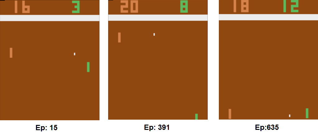
And, truth be told, our trained model is pretty darn good at Pong. Take a look:

Yes, I know someone already wrote a 130-lines-of-Python algorithm (with very limited dependencies) that solves Pong. But, that was back in 2016, and it took him 3 whole nights on his MacBook to train the model.

In 2018, we can use Keras, along with cutting edge GPUs on FloydHub, to train our Pong AI effortlessly.

Let’s get started.

Psst.

All the code in this post is available on GitHub in Jupyter notebooks, if you’d like to follow along. Also, if you're new to deep learning, I'd recommend getting a feel for things by checking out Emil’s Deep Learning tutorial.

One more thing – the name of the guy who wrote the 130 lines of Python Pong AI?

Andrej Karpathy, now director of AI at Tesla.

Now back to your regularly scheduled program.

Setting up our Deep RL environment

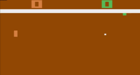
Before we go any further, let's run a quick demo to get a sense of what our environment looks like. We'll build a Pong bot that moves randomly, much like my younger niece does while exploring the world.

Note: The key component of the whole process is our gym environment Pong-v0, so please, make sure you put your gym seatbelt on (HINT: pip install gym). If you're using my GitHub repo on FloydHub, gym will be installed automatically when you start your Workspace.

Let's start by initializing our Pong environment:

import gym
import random

# code for the two only actions in Pong
UP_ACTION = 2
DOWN_ACTION = 3

# initializing our environment
env = gym.make("Pong-v0")

# beginning of an episode
observation = env.reset()

What's happening here?

• We're initializing our environment env using Pong-v0 from gym default environments, and using reset to initialize it.
• We're declaring our potential actions. If you’ve ever played Pong, then you’ll remember that there only two actions you can perform: moving up and moving down. That’s it.

And now, the showstopper:

# main loop
for i in range(300):
    # render a frame
    env.render()

    # choose random action
    action = random.randint(UP_ACTION, DOWN_ACTION) 

    # run one step
    observation, reward, done, info = env.step(action)

    # if the episode is over, reset the environment
    if done:
        env.reset()

PS: if you’re running the demo from my Jupyter notebook, I’ve added some code there to save the frames as a gif, because it’s not possible to load the GUI inside a Jupyter notebook.

After running this code, you'll see our Pong agent playing randomly, like this:

We can do better. Next up, I’ll show you how to code an AI that can do better than random, using Reinforcement Learning.

Reinforcement Learning Overview

Time for a few quick definitions. In Reinforcement Learning, an agent perceives its environment through observations and rewards, and acts upon it through actions.

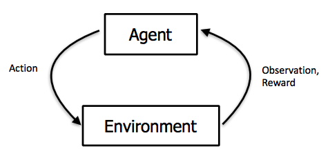
The agent learns which actions maximize the reward, given what it learned from the environment.

More precisely, in our Pong case:

• The agent is the Pong AI model we’re training.
• The action is the output of our model: tells if the paddle should go up or down.
• The environment is everything that determines the state of the game.
• The observation is what the agent sees from the environment (here, the frames).
• The reward is what our agent gains after taking an action in the environment (here losing -1 after missing the ball, +1 if the opponent missed the ball).

Note: The reward in our Pong environment will actually be zero for most of the steps in our environment, because no point is scored at that moment (i.e. no player misses the ball).

Goal Setting

Let's recap our goal. We want our AI to learn Pong... from scratch.

That's right. Our AI doesn't know the rules of the game. It doesn't even know what a ball is.

Its input is simply the sequence of frames it gets from observations.

Its output is a policy – a set of rules that say what to do in every situation.

Let's imagine we're the agent (green paddle on the right) in this situation. If you see the following sequence of frames, what do you do?

You continue to go down to stop the ball, right?

Your brain (i.e. your 10^11 neural network) correctly predicted the best move.

Congrats!

Now, we'll train a much smaller neural net to predict the same thing.

Neural Network

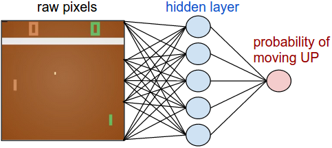
We'll use a simple Neural Network, with only one 200-units hidden layer:

In Keras, we initialize our model as follow:

# import necessary modules from keras
from keras.layers import Dense
from keras.models import Sequential

# creates a generic neural network architecture
model = Sequential()

# hidden layer takes a pre-processed frame as input, and has 200 units
model.add(Dense(units=200,input_dim=80*80, activation='relu', kernel_initializer='glorot_uniform'))

# output layer
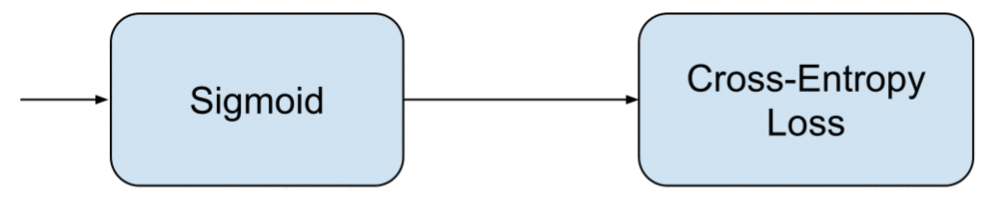
model.add(Dense(units=1, activation='sigmoid', kernel_initializer='RandomNormal'))

# compile the model using traditional Machine Learning losses and optimizers
model.compile(loss='binary_crossentropy', optimizer='adam', metrics=['accuracy'])

A couple of things to notice here:

• The 80 * 80 input dimension comes from the pre-processing of the raw pixels made by Karpathy (the only important pixels are the balls and the paddle). Actually, we'll feed the pre-processed version of the difference between the current frame and the last frame to express things like the direction of the ball.

The result of the difference of the two last frames input depends on the order of the two frames (frame1 - frame2 != frame2 - frame1). Thus, that difference encodes the position of the ball for two frames and the order between those frames, which gives you the direction of the ball. The awesome thing about using neural networks is that they automatically detects regularities in the input. Adjusting the weights between the input (frames) and the hidden layer, our neural network will incorporate such regularities (like the direction of a ball) into the model.

Here is a visualization of 300 inputs (pre-processed difference of frames) in black and white (cf. demo_black_and_white.ipynb):

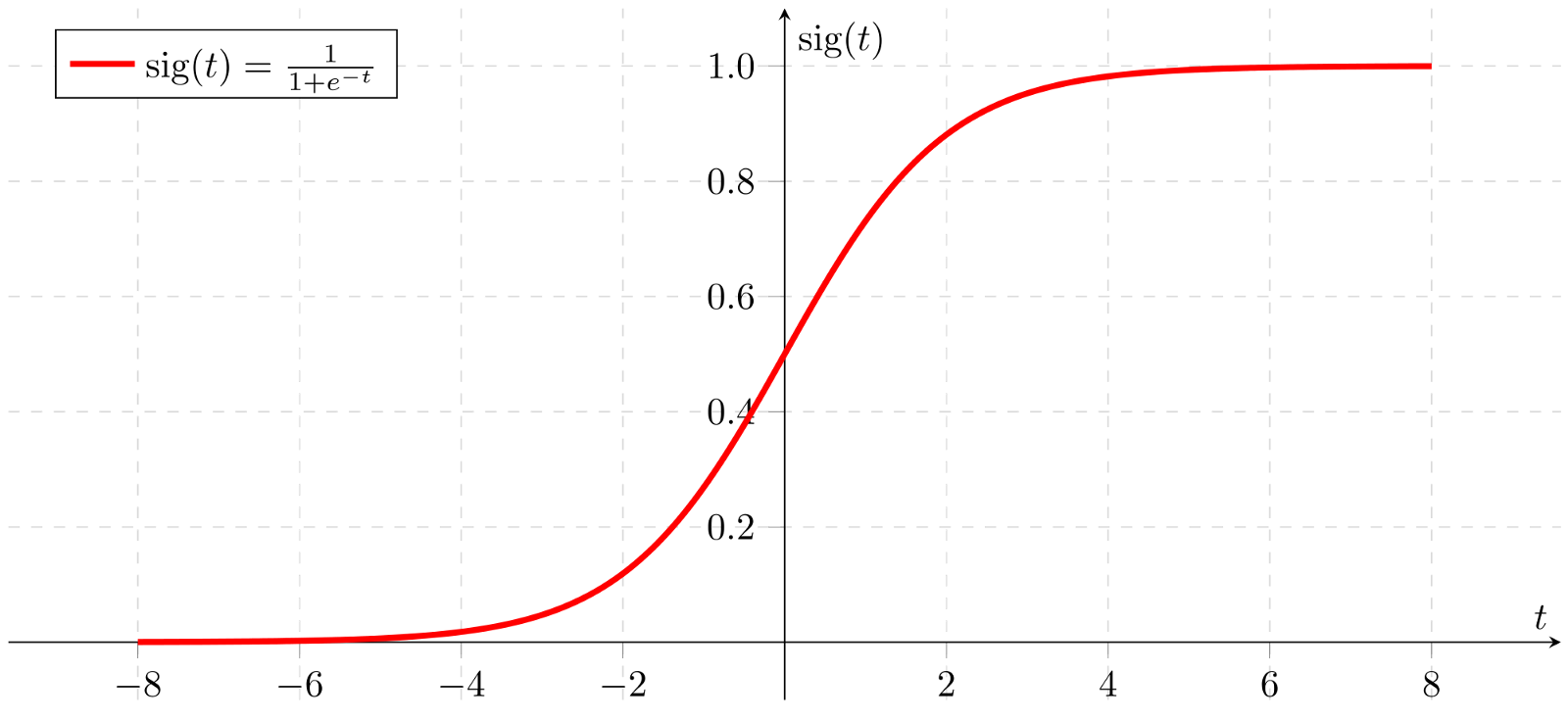
• A sigmoid activation is used for the output layer because it must predict a probability of choosing the action UP (sigmoid is between 0 and 1)

• Then, we use the binary_crossentropy loss (standard loss for classification problems) because, at the end of the day, we want to assign the different pre-processed frames either the class move UP or move DOWN.

Vanilla Policy Gradient

Let's come back to our initial goal: implementing a Vanilla Policy Gradient, following OpenAI's Spinning Up guide.

We just coded a neural network that outputs a probability of moving up, defining a policy (that tells what actions to take in every situation). More generally, Policy Gradient methods aim at directly finding the best policy in policy-space, and a Vanilla Policy Gradient is just a basic implementation.

The gradient part comes from the optimization process, that usually involves something like gradient descent, when tuning a set of parameters (here the weights of our neural network).

Learning

Before attacking the core of the learning, let's see where we are in our to-do list:

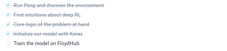
Almost there, right?

Training our Deep RL Model

FloydHub is a training platform for deep learning. I came across them reading Matthew Rahtz's blogpost about reproducing deep RL papers. That's how he explained his choice of FloydHub over Compute Engine:

Compute Engine is fine if you just want shell access to a GPU machine, but I tried to do as much as possible on FloydHub. FloydHub is basically a cloud compute service targeted at machine learning. You run floyd run python awesomecode.py and FloydHub sets up a container, uploads your code to it, and runs the code. The two key things which make FloydHub awesome are:

• Containers come preinstalled with GPU drivers and common libraries. (Even in 2018, [he] wasted a good few hours fiddling with CUDA versions while upgrading TensorFlow on the Compute Engine VM.)
• Each run is automatically archived. For each run, the code used, the exact command used to start the run, any command-line output, and any data outputs are saved automatically, and indexed through a web interface.

His conclusion?

Unless your budget is really limited, the extra convenience of FloydHub is worth it.

It also makes it extra convenient to share your Machine Learning projects, like this one.

Setting things up

1. If you are new to FloydHub, start with their 2-min installation
2. Create a new project
3. Inside your project, click on the Workspaces tab, and then on Create Workspace
4. At this point, click on Import from GitHub and enter the following url: https://github.com/mtrazzi/spinning-up-a-Pong-AI-with-deep-RL. Normally, after a few seconds, your ready Workspace should appear
5. After clicking on Files on the left, click on the file train.ipynb

That's it! You've just accessed a Jupyter-notebook-compatible fully-fledged environment.

You can also reproduce all those steps by just clicking this button - trust me, it's much easier this way:

Model training logic

If you followed steps 1 to 7, you can now see the Jupyter notebook train.ipynb:

• First cell: initialization of the keras model (cf. the "Neural Network" part).
• Second cell: initialization of our gym environment.
• Third cell: main loop where everything happens.

Intuition

In Supervised Learning, you get to train your algorithm on labeled data before you test it. Reinforcement Learning also uses training data, and can be very similar to Supervised Learning in this respect – but there's a big difference:

There is no labeled data with Reinforcement Learning.

In the magic world of Reinforcement Learning, that's fine! We separate the training phases into episodes, where an episode is just the sequence of frames from the beginning of a game (no player has scored yet) to the end of the game (one player has won the Pong match because that player reached 21 points first).

For each episode, we first generate the data, and then train our algorithm using this data.

Code

Let’s look inside the main loop. Here's what happens for every step of the algorithm (i.e. frame of the game):

1. We start by preprocessing the observation frame, and then doing the difference with the previous frame.

# preprocess the observation, set input as difference between images
cur_input = prepro(observation)
x = cur_input - prev_input if prev_input is not None else np.zeros(80 * 80)
prev_input = cur_input

2. Running model.predict to know what the current model thinks about the probability of doing the UP_ACTION, given the current frame setting.

# forward the policy network and sample action according to the proba distribution
proba = model.predict(np.expand_dims(x, axis=1).T)

3. Sampling the next action using the probability outputted above.

action = UP_ACTION if np.random.uniform() < proba else DOWN_ACTION

4. Adding a label y in y_train for the input x corresponding to this action (will be used in training).

y = 1 if action == UP_ACTION else 0 # 0 and 1 are our labels

# log the input and label to train later
x_train.append(x)
y_train.append(y)

5. Running one step of the game (i.e. go from current frame to the next frame, by using either action UP or DOWN) with env.step(action), logging the reward.

	# do one step in our environment
	observation, reward, done, info = env.step(action)
	rewards.append(reward)
	reward_sum += reward

6. Additionally, if it’s the end of a game (one player has reached 21), we train the model with the generated data using model.fit, and all the gathered data (x_train,y_train, reward).

    # end of an episode
    if done:
        print('At the end of episode', episode_nb, 'the total reward was :', reward_sum)
        # increment episode number
        episode_nb += 1
        
        # training
        model.fit(x=np.vstack(x_train), y=np.vstack(y_train), verbose=1, sample_weight=discount_rewards(rewards, gamma))

And then reinitializes everything:

        # Reinitialization
        x_train, y_train, rewards = [],[],[]
        observation = env.reset()
        reward_sum = 0
        prev_input = None

The training part in model.fit works as follows:

• If an action leads to a positive reward, it tunes the weights of the neural network so it keeps on predicting this winning action.
• Otherwise, it tunes them in the opposite way
• The function discount_rewards transforms the list of rewards so that even actions that remotely lead to positive rewards are encouraged.

Some examples to make it more concrete:

• x_train[frame_number] : mostly zero, with occasional 1 or -1 after pre-processing/difference between frames.

…0.0 0.0 0.0 0.0 0.0 0.0 0.0 0.0 0.0 0.0 0.0 0.0 0.0 0.0 0.0 0.0 0.0 0.0 0.0 0.0 0.0 0.0 0.0 0.0 0.0 0.0 0.0 0.0 0.0 0.0 0.0 0.0 0.0 0.0 0.0 0.0 0.0 0.0 -1.0 -1.0 0.0 0.0 0.0 0.0 0.0 0.0 0.0 0.0 0.0 0.0 0.0 0.0 0.0 0.0 0.0 0.0 0.0 0.0 0.0 0.0 0.0 0.0 0.0 0.0 0.0…

• y_train : only zeros (for DOWN_ACTION) and ones (for UP_ACTION)

[0, 0, 1, 0, 1, 1, 0, 1, 1, 0, 1, 1, 0, 1, 0, 1, 0, …, 0, 1, 1, 0, 1, 1, 1, 0]

• rewards : to each frame (x_train[frame_number]) and action (y_train[frame_number]) is associated a reward (-1 if it missed the ball, 0 if nothing happens, and 1 if opponent misses the ball), so we get for instance the following array:

...0.0, 0.0, 0.0, 0.0, 0.0, 0.0, 0.0, 0.0, 0.0, 0.0, 0.0, 0.0, 0.0, 0.0, 0.0, 0.0, -1.0, 0.0, 0.0, 0.0, 0.0, 0.0, 0.0, 0.0, 0.0, 0.0, 0.0, 0.0, 0.0, 0.0, 0.0, 0.0, 0.0, 0.0, 0.0, 0.0, 0.0, 0.0, 0.0, 0.0, 0.0, 0.0, 0.0, 0.0, 0.0, 1.0…

• the discounted rewards after applying discount_rewards (the negative rewards are spread to the frames before our model missed the ball (before the -1.0 in reward), idem for the positive.

...-1.22 -1.23 -1.24 -1.25 -1.26 -1.27 -1.28 -1.29 -1.3  -1.31 -1.32 -1.33
 -1.34 -1.36 -1.37 -1.38 -1.39  0.63  0.64  0.65  0.66  0.66  0.67  0.68
  0.69  0.7   0.71  0.72  0.73  0.74  0.75  0.76  0.77  0.78  0.79  0.8
  0.81  0.82  0.83  0.84  0.85  0.87  0.88  0.89  0.9   0.91...

Let’s put this into practice.

Running the notebook

To run the notebook, click on the Run tab at the top of the workspace, then on Run all cells.

If everything goes according to the plan, you'll see the following output:

At the end of episode 0 the total reward was : -20.0
Epoch 1/1
1225/1225 [==============================] - 0s 359us/step - loss: -0.0015 - acc: 0.4816
At the end of episode 1 the total reward was : -21.0
Epoch 1/1
1102/1102 [==============================] - 0s 153us/step - loss: -0.0094 - acc: 0.5327
...

If that's the case, congrats! You can interrupt the kernel. (The goal here was just to run the training for a few epochs to get a feel of how the process works. The actual training takes several hours). As you can see, we're tracking the reward gained after each Pong episode.

The first player to win 21 games wins the episode. That means that a reward of -20.0 corresponds to our AI losing 21 games and winning only one.

The algorithm needs thousands of episodes to actually learn something. You'll probably want to plot the data from our learning to track how things are going. Fortunately, I prepared everything for you on another notebook.

Plotting the Results with TensorBoard and FloydHub

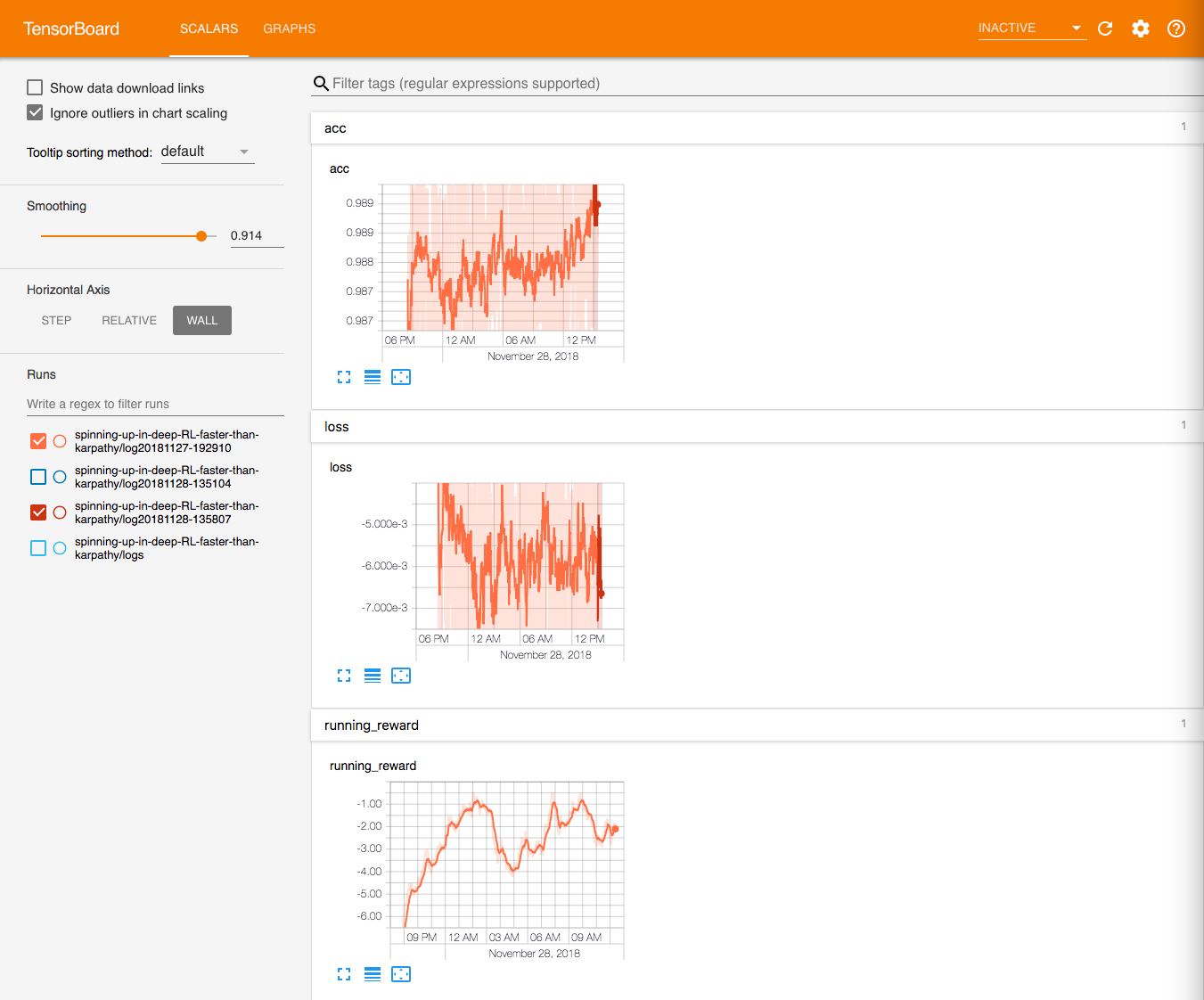
Go back to your FloydHub Workspace, and open the notebook train-with-log.ipynb. Then, run the notebook (click on the Run tab at the top of the workspace, then on Run all cells). Now, click on the TensorBoard link (inside the blue dashboard bar at the bottom of the screen).

After clicking on the link, FloydHub automatically detects all the TensorBoard logs repositories. You should be seeing a window that looks like this (click on Wall to see the following acc and loss graph):

The notebook train-with-log.ipynb is just the old train.ipynb with additional lines of code to log some variables and metrics.

With Keras, it involves creating a callback object:

tbCallBack = callbacks.TensorBoard(log_dir=log_dir, histogram_freq=0, write_graph=True, write_images=True)

And calling the tbCallBack object when training:

model.fit(x=np.vstack(x_train), y=np.vstack(y_train), verbose=1, callbacks=[tbCallBack], sample_weight=discount_rewards(rewards, gamma))

I also used an additional function tflog to easily keep track of variables not related to Keras, like the running_reward (=smoothed reward). After having imported the file containing the function, calling it is as simple as:

tflog('running_reward', running_reward)

Training

Training the Keras model to achieve Karpathy’s results (i.e. winning about half the games, or a reward of 0) took about 30 hours of training and 10,000 episodes.

To train, I used FloydHub’s Standard GPU Tesla K80. This allowed me to start the training instantly with almost zero setup. I would do sanity checks on my phone and the training would continue effortlessly for hours.

Also, Keras made it super easy to save and load models (cf. the train-with-log.ipynb notebook). To save and load weights, just do the following commands:

model.save_weights('current_weights.h5')
model.load_weights('old_weights.h5')

It looks like we achieved results similar from Karpathy’s in about the same time (he trained his model for three nights).

However, setting everything up took some time and debugging.

In most practical cases, it is common to experiment with different models before choosing one in particular, and it is a costly process to implement each one by yourself. In 2018, more and more Deep RL frameworks are open-sourced, and allow non-expert to smoothly carry out experiments using efficient implementations.

For our next step, we’ll be trying out one of those Deep RL framework to test how our Keras model compares to a standard implementation of Policy Gradient, and experiment how easy it is to start getting results.

We'll be using OpenAI’s Spinning Up into Deep RL resource.

Using OpenAI's Spinning Up

On November 8th, OpenAI released their educational package to let anyone get started in Deep RL.

Can it help us master Pong?

Let’s start with the setup of “spinning up” on FloydHub, and then we’ll try to use it for our task.

Setting up

1. Go back to your project page, and create a new Workspace (click on Create Workspace).
2. Select Import from Github and enter the url https://github.com/mtrazzi/spinningup
3. Choose TensorFlow 1.10 and the best hardware you have (works best on GPU)
4. Normally, after a few seconds, your ready Workspace should appear

Again, you can just click this button to bootstrap your Workspace:

Now, a few more steps to do, since we’ll be working in the Terminal of the FloydHub workspace:

1. Click on the Launcher tab, and open a new Terminal (at the bottom)
2. Launch the command pip install -U -e  .
3. While it’s installing, go to your Settings (expanding on the right, clicking on Settings) and select Disable idle timeout in “Idle Timeout”. This avoids your terminal experiments to be shutdown.

Training

To launch the training, run the following command in the terminal:

python -m spinup.run vpg --hid "[200]" --env Pong-ram-v0 --exp_name FloydHub-blog --dt --epochs 20000 --seed 40

You should be seeing a series of outputs similar to this:

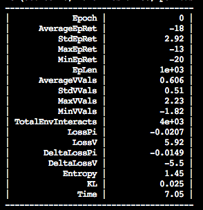
What's going on here?

We’re running the algorithm vpg or “vanilla policy gradient”, with a 200-units hidden layer, on the environment Pong-ram-v0, for 20 000 episodes (=20 000 epochs here), and with an initial seed of 40 (the seed is a parameter that controls the initialization of the gym environment).

Basically, we’re doing something similar to what we were doing previously in Keras (i.e. training the same neural network with a simple policy gradient algorithm), without having to code anything, directly from the command line!

Additionally, we get a bunch of real-time metrics outputted for free, and that’s priceless for debugging.

The key metric is the AverageEpRet, or average reward for the Epoch.

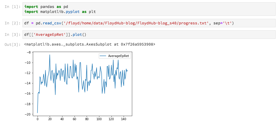
Plotting the results

Spinning Up makes it super easy to plot the results by automatically saving the results in .csv files. The following is a standard way of plotting such results.

After a few iterations, enter the notebooks folder (on the left), and click on plot.ipynb. Now click on Rull All Cells (after clicking on the Run tab, at the top).

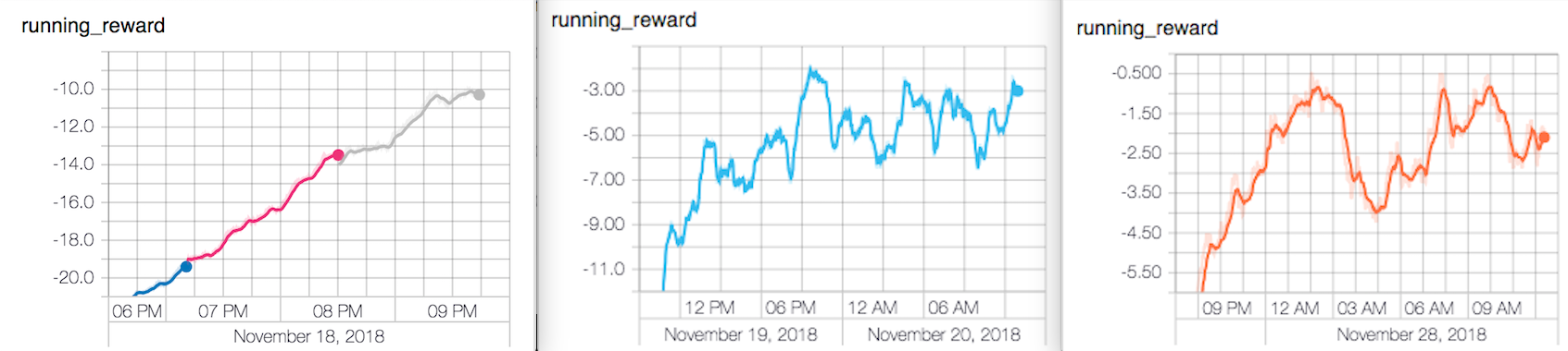
You should be facing something similar to this:

Cool!

With a minimal setup, our algorithm is already quickly learning something.

Here is what you get after more iterations:

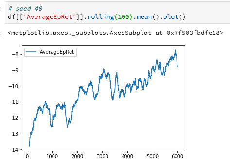
It is taking more episodes to train than our Keras model (we reached the same result in only ~2000 episodes). However, we're using an out-of-the-box “vanilla policy gradient” from the “Spinning Up” repository, and there is no ad hoc pre-processing required.

Conclusion

In short, using the spinning up repo with FloydHub completely transformed the experience of running experiments into something effortless.

Yes, we’re still far away from solving Pong in 30 minutes:

• There is still room for improvement for the Keras model (e.g. by tuning the learning rate).
• It is possible to parallelize the episode runs by launching multiple episodes in parallel and then training the model with the obtained data.

Yet, with Keras, we achieved results similar to Karpathy’s, and now with OpenAI’s repo, we’re able to experiment faster than ever before.

In other words, we’re taking deep RL for a spin.

Thanks to Emil Wallner for helping me debug my Keras models, Charlie Harrington for his feedback, and the FloydHub team for letting me run my trainings on their servers.

FloydHub Call for AI writers

Want to write amazing articles like Michaël and play your role in the long road to Artificial General Intelligence? We are looking for passionate writers, to build the world's best blog for practical applications of groundbreaking A.I. techniques. FloydHub has a large reach within the AI community and with your help, we can inspire the next wave of AI. Apply now and join the crew!

About Michaël Trazzi

This is the first in a series of articles by Michaël Trazzi documenting his journey into Deep Reinforcement Learning. Michaël codes at 42 and is finishing a Master's Degree in AI. He's currently exploring the limits of productivity and the future of AI. Michaël is also a FloydHub AI Writer.

You can follow along with Michaël on Medium, Twitter and Github.