Long Short-Term Memory: From Zero to Hero with PyTorch
Long Short-Term Memory (LSTM) Networks have been widely used to solve various sequential tasks. Let's find out how these networks work and how we can implement them.


Just like us, Recurrent Neural Networks (RNNs) can be very forgetful. This struggle with short-term memory causes RNNs to lose their effectiveness in most tasks. However, do not fret, Long Short-Term Memory networks (LSTMs) have great memories and can remember information which the vanilla RNN is unable to!
LSTMs are a particular variant of RNNs, therefore having a grasp of the concepts surrounding RNNs will significantly aid your understanding of LSTMs in this article. I covered the mechanism of RNNs in my previous article here.
A quick recap on RNNs
RNNs process inputs in a sequential manner, where the context from the previous input is considered when computing the output of the current step. This allows the neural network to carry information over different time steps rather than keeping all the inputs independent of each other.
However, a significant shortcoming that plagues the typical RNN is the problem of vanishing/exploding gradients. This problem arises when back-propagating through the RNN during training, especially for networks with deeper layers. The gradients have to go through continuous matrix multiplications during the back-propagation process due to the chain rule, causing the gradient to either shrink exponentially (vanish) or blow up exponentially (explode). Having a gradient that is too small prevents the weights from updating and learning, whereas extremely large gradients cause the model to be unstable.
Due to these issues, RNNs are unable to work with longer sequences and hold on to long-term dependencies, making them suffer from “short-term memory”.
What are LSTMs
While LSTMs are a kind of RNN and function similarly to traditional RNNs, its Gating mechanism is what sets it apart. This feature addresses the “short-term memory” problem of RNNs.
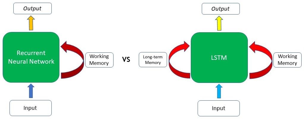
As we can see from the image, the difference lies mainly in the LSTM’s ability to preserve long-term memory. This is especially important in the majority of Natural Language Processing (NLP) or time-series and sequential tasks. For example, let’s say we have a network generating text based on some input given to us. At the start of the text, it is mentioned that the author has a “dog named Cliff”. After a few other sentences where there is no mention of a pet or dog, the author brings up his pet again, and the model has to generate the next word to "However, Cliff, my pet ____". As the word pet appeared right before the blank, a RNN can deduce that the next word will likely be an animal that can be kept as a pet.
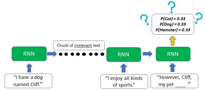
However, due to the short-term memory, the typical RNN will only be able to use the contextual information from the text that appeared in the last few sentences - which is not useful at all. The RNN has no clue as to what animal the pet might be as the relevant information from the start of the text has already been lost.
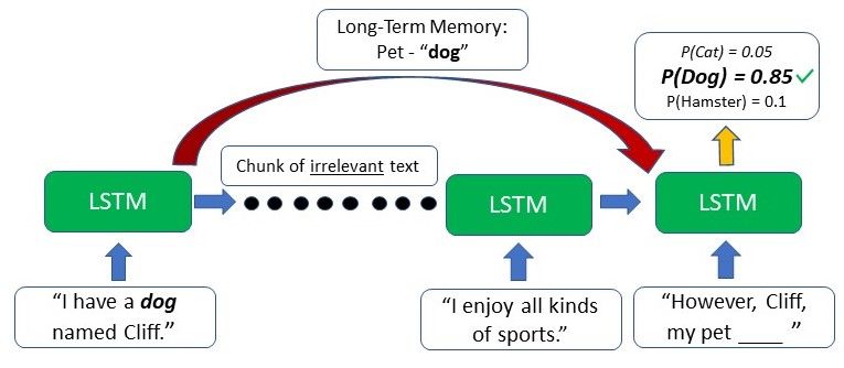
On the other hand, the LSTM can retain the earlier information that the author has a pet dog, and this will aid the model in choosing "the dog" when it comes to generating the text at that point due to the contextual information from a much earlier time step.
Inner workings of the LSTM
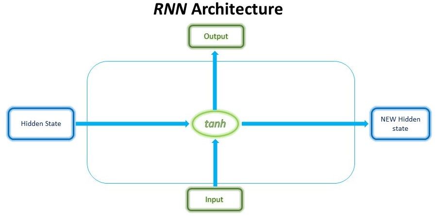
The secret sauce to the LSTM lies in its gating mechanism within each LSTM cell. In the normal RNN cell, the input at a time-step and the hidden state from the previous time step is passed through a tanh activation function to obtain a new hidden state and output.
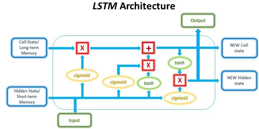
LSTMs, on the other hand, have a slightly more complex structure. At each time step, the LSTM cell takes in 3 different pieces of information -- the current input data, the short-term memory from the previous cell (similar to hidden states in RNNs) and lastly the long-term memory.
The short-term memory is commonly referred to as the hidden state, and the long-term memory is usually known as the cell state.
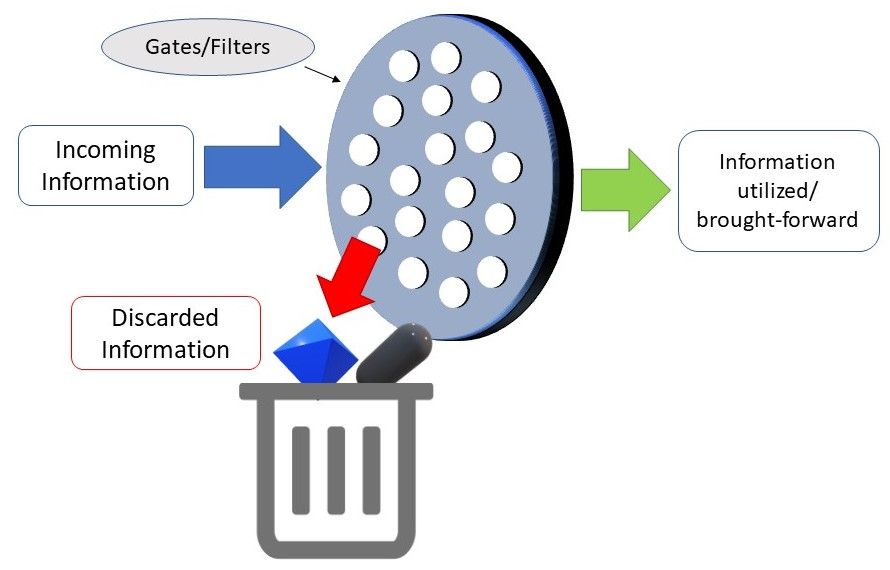
The cell then uses gates to regulate the information to be kept or discarded at each time step before passing on the long-term and short-term information to the next cell.
These gates can be seen as water filters. Ideally, the role of these gates is supposed to selectively remove any irrelevant information, similar to how water filters prevent impurities from passing through. At the same time, only water and beneficial nutrients can pass through these filters, just like how the gates only hold on to the useful information. Of course, these gates need to be trained to accurately filter what is useful and what is not.
These gates are called the Input Gate, the Forget Gate, and the Output Gate. There are many variants to the names of these gates; nevertheless, the calculations and workings of these gates are mostly the same.
Let’s go through the mechanisms of these gates one-by-one.
Input Gate
The input gate decides what new information will be stored in the long-term memory. It only works with the information from the current input and the short-term memory from the previous time step. Therefore, it has to filter out the information from these variables that are not useful.
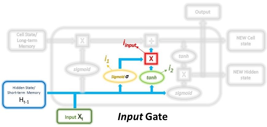
Mathematically, this is achieved using 2 layers. The first layer can be seen as the filter which selects what information can pass through it and what information to be discarded. To create this layer, we pass the short-term memory and current input into a sigmoid function. The sigmoid function will transform the values to be between 0 and 1, with 0 indicating that part of the information is unimportant, whereas 1 indicates that the information will be used. This helps to decide the values to be kept and used, and also the values to be discarded. As the layer is being trained through back-propagation, the weights in the sigmoid function will be updated such that it learns to only let the useful pass through while discarding the less critical features.
$$i_1 = \sigma(W_{i_1} \cdot (H_{t-1}, x_t) + bias_{i_1})$$
The second layer takes the short term memory and current input as well and passes it through an activation function, usually the $$tanh$$ function, to regulate the network.
$$i_2 = tanh(W_{i_2} \cdot (H_{t-1}, x_t) + bias_{i_2})$$
The outputs from these 2 layers are then multiplied, and the final outcome represents the information to be kept in the long-term memory and used as the output.
$$i_{input} = i_1 * i_2$$
Forget Gate
The forget gate decides which information from the long-term memory should be kept or discarded. This is done by multiplying the incoming long-term memory by a forget vector generated by the current input and incoming short-term memory.
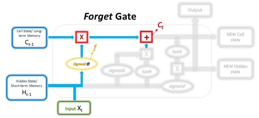
Just like the first layer in the Input gate, the forget vector is also a selective filter layer. To obtain the forget vector, the short-term memory, and current input is passed through a sigmoid function, similar to the first layer in the Input Gate above, but with different weights. The vector will be made up of 0s and 1s and will be multiplied with the long-term memory to choose which parts of the long-term memory to retain.
$$f = \sigma(W_{forget} \cdot (H_{t-1}, x_t) + bias_{forget})$$
The outputs from the Input gate and the Forget gate will undergo a pointwise addition to give a new version of the long-term memory, which will be passed on to the next cell. This new long-term memory will also be used in the final gate, the Output gate.
$$C_t = C_{t-1} * f + i_{input}$$
Output Gate
The output gate will take the current input, the previous short-term memory, and the newly computed long-term memory to produce the new short-term memory/hidden state which will be passed on to the cell in the next time step. The output of the current time step can also be drawn from this hidden state.
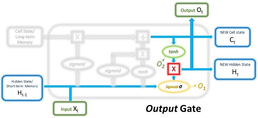
First, the previous short-term memory and current input will be passed into a sigmoid function (Yes, this is the 3rd time we’re doing this) with different weights yet again to create the third and final filter. Then, we put the new long-term memory through an activation $$tanh$$ function. The output from these 2 processes will be multiplied to produce the new short-term memory.
$$O_1 = \sigma (W_{output_1} \cdot (H_{t-1}, x_t) + bias_{output_1})$$
$$O_2 = tanh(W_{output_2} \cdot C_t + bias_{output_2})$$
$$H_t, O_t = O_1 * O_2$$
The short-term and long-term memory produced by these gates will then be carried over to the next cell for the process to be repeated. The output of each time step can be obtained from the short-term memory, also known as the hidden state.
That's all there is to the mechanisms of the typical LSTM structure. Not all that tough, eh?
Code Implementation
With the necessary theoretical understanding of LSTMs, let's start implementing it in code. We'll be using the PyTorch library today.
Before we jump into a project with a full dataset, let's just take a look at how the PyTorch LSTM layer really works in practice by visualizing the outputs. We don't need to instantiate a model to see how the layer works. You can run this on FloydHub with the button below under LSTM_starter.ipynb. (You don’t need to run on a GPU for this portion)

import torch
import torch.nn as nn
Just like the other kinds of layers, we can instantiate an LSTM layer and provide it with the necessary arguments. The full documentation of the accepted arguments can be found here. In this example, we will only be defining the input dimension, hidden dimension, and the number of layers.
- Input dimension - represents the size of the input at each time step, e.g. input of dimension 5 will look like this [1, 3, 8, 2, 3]
- Hidden dimension - represents the size of the hidden state and cell state at each time step, e.g. the hidden state and cell state will both have the shape of [3, 5, 4] if the hidden dimension is 3
- Number of layers - the number of LSTM layers stacked on top of each other
input_dim = 5
hidden_dim = 10
n_layers = 1

lstm_layer = nn.LSTM(input_dim, hidden_dim, n_layers, batch_first=True)
Let's create some dummy data to see how the layer takes in the input. As our input dimension is 5, we have to create a tensor of the shape (1, 1, 5) which represents (batch size, sequence length, input dimension).
Additionally, we'll have to initialize a hidden state and cell state for the LSTM as this is the first cell. The hidden state and cell state is stored in a tuple with the format (hidden_state, cell_state).
batch_size = 1
seq_len = 1

inp = torch.randn(batch_size, seq_len, input_dim)
hidden_state = torch.randn(n_layers, batch_size, hidden_dim)
cell_state = torch.randn(n_layers, batch_size, hidden_dim)
hidden = (hidden_state, cell_state)
[Out]:
Input shape: (1, 1, 5)
Hidden shape: ((1, 1, 10), (1, 1, 10))
Next, we’ll feed the input and hidden states and see what we’ll get back from it.
out, hidden = lstm_layer(inp, hidden)
print("Output shape: ", out.shape)
print("Hidden: ", hidden)
[Out]: Output shape: torch.size([1, 1, 10])
	 Hidden: (tensor([[[ 0.1749,  0.0099, -0.3004,  0.2846, -0.2262, -0.5257,  0.2925, -0.1894,  0.1166, -0.1197]]], grad_fn=<StackBackward>), tensor([[[ 0.4167,  0.0385, -0.4982,  0.6955, -0.9213, -1.0072,  0.4426,
          -0.3691,  0.2020, -0.2242]]], grad_fn=<StackBackward>))
In the process above, we saw how the LSTM cell will process the input and hidden states at each time step. However in most cases, we'll be processing the input data in large sequences. The LSTM can also take in sequences of variable length and produce an output at each time step. Let's try changing the sequence length this time.
seq_len = 3
inp = torch.randn(batch_size, seq_len, input_dim)
out, hidden = lstm_layer(inp, hidden)
print(out.shape)
[Out]: torch.Size([1, 3, 10])
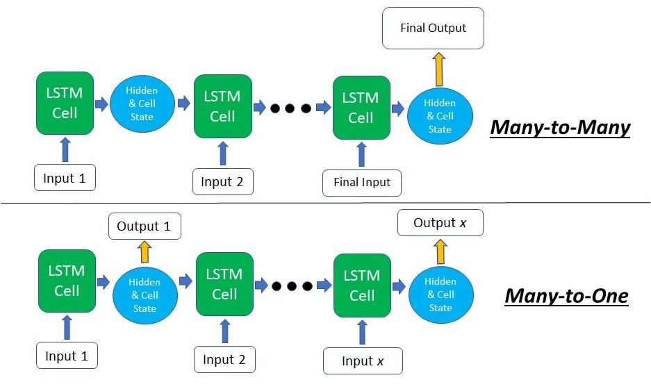
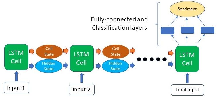
This time, the output's 2nd dimension is 3, indicating that there were 3 outputs given by the LSTM. This corresponds to the length of our input sequence. For the use cases where we'll need an output at every time step (many-to-many), such as Text Generation, the output of each time step can be extracted directly from the 2nd dimension and fed into a fully connected layer. For text classification tasks (many-to-one), such as Sentiment Analysis, the last output can be taken to be fed into a classifier.
# Obtaining the last output
out = out.squeeze()[-1, :]
print(out.shape)
[Out]: torch.Size([10])
Project: Sentiment Analysis on Amazon Reviews
For this project, we’ll be using the Amazon customer reviews dataset which can be found on Kaggle. The dataset contains a total of 4 million reviews with each review labeled to be of either positive or negative sentiment. You can run the code implementation in this article on FloydHub using their GPUs on the cloud by clicking the following link and using the main.ipynb notebook.
This will speed up the training process significantly. Alternatively, the link to the GitHub repository can be found here.
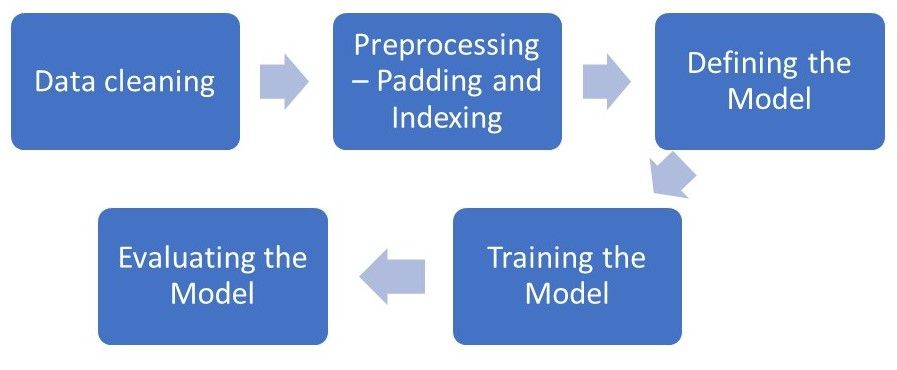
Our goal at the time of this implementation will be to create an LSTM model that can accurately classify and distinguish the sentiment of a review. To do so, we’ll have to start with some data-preprocessing, defining and training the model, followed by assessing the model.
The process flow of our implementation looks like this.
We will only be using 1 million reviews in this implementation to speed things up, however, feel free to run it yourself with the entire dataset if you have the time and computing capacity.
For our data pre-processing steps, we'll be using regex, Numpy and the NLTK (Natural Language Toolkit) library for some simple NLP helper functions. As the data is compressed in the bz2 format, we'll use the Python bz2 module to read the data.
import bz2
from collections import Counter
import re
import nltk
import numpy as np
nltk.download('punkt')

train_file = bz2.BZ2File('../input/amazon_reviews/train.ft.txt.bz2')
test_file = bz2.BZ2File('../input/amazon_reviews/test.ft.txt.bz2')

train_file = train_file.readlines()
test_file = test_file.readlines()
Number of training reviews: 3600000
Number of test reviews: 400000
This dataset contains a total of 4 million reviews - 3.6 million training and 0.4 million for testing. We will be using only 800k for training and 200k for testing here -- this is still a large amount of data.
num_train = 800000  # We're training on the first 800,000 reviews in the dataset
num_test = 200000  # Using 200,000 reviews from test set

train_file = [x.decode('utf-8') for x in train_file[:num_train]]
test_file = [x.decode('utf-8') for x in test_file[:num_test]]
The format of the sentences are as such:__label__2 Stunning even for the non-gamer: This soundtrack was beautiful! It paints the scenery in your mind so well I would recommend it even to people who hate vid. game music! I have played the game Chrono Cross but out of all of the games I have ever played it has the best music! It backs away from crude keyboarding and takes a fresher step with great guitars and soulful orchestras. It would impress anyone who cares to listen! ^_^
We'll have to extract out the labels from the sentences. The data is the format __label__1/2 <sentence>, therefore we can easily split it accordingly. Positive sentiment labels are stored as 1 and negative are stored as 0.
We will also change all URLs to a standard <url\> as the exact URL is irrelevant to the sentiment in most cases.
# Extracting labels from sentences
train_labels = [0 if x.split(' ')[0] == '__label__1' else 1 for x in train_file]
train_sentences = [x.split(' ', 1)[1][:-1].lower() for x in train_file]

test_labels = [0 if x.split(' ')[0] == '__label__1' else 1 for x in test_file]
test_sentences = [x.split(' ', 1)[1][:-1].lower() for x in test_file]

# Some simple cleaning of data
for i in range(len(train_sentences)):
    train_sentences[i] = re.sub('\d','0',train_sentences[i])

for i in range(len(test_sentences)):
    test_sentences[i] = re.sub('\d','0',test_sentences[i])

# Modify URLs to <url>
for i in range(len(train_sentences)):
    if 'www.' in train_sentences[i] or 'http:' in train_sentences[i] or 'https:' in train_sentences[i] or '.com' in train_sentences[i]:
        train_sentences[i] = re.sub(r"([^ ]+(?<=\.[a-z]{3}))", "<url>", train_sentences[i])

for i in range(len(test_sentences)):
    if 'www.' in test_sentences[i] or 'http:' in test_sentences[i] or 'https:' in test_sentences[i] or '.com' in test_sentences[i]:
        test_sentences[i] = re.sub(r"([^ ]+(?<=\.[a-z]{3}))", "<url>", test_sentences[i])
After quickly cleaning the data, we will do tokenization of the sentences, which is a standard NLP task.
Tokenization is the task of splitting a sentence into individual tokens, which can be words or punctuation, etc.
There are many NLP libraries that can do this, such as spaCy or Scikit-learn, but we will be using NLTK here as it has one of the faster tokenizers.
The words will then be stored in a dictionary mapping the word to its number of appearances. These words will become our vocabulary.
words = Counter()  # Dictionary that will map a word to the number of times it appeared in all the training sentences
for i, sentence in enumerate(train_sentences):
    # The sentences will be stored as a list of words/tokens
    train_sentences[i] = []
    for word in nltk.word_tokenize(sentence):  # Tokenizing the words
        words.update([word.lower()])  # Converting all the words to lowercase
        train_sentences[i].append(word)
    if i%20000 == 0:
        print(str((i*100)/num_train) + "% done")
print("100% done")
- To remove typos and words that likely don't exist, we'll remove all words from the vocab that only appear once throughout.
- To account for unknown words and padding, we'll have to add them to our vocabulary as well. Each word in the vocabulary will then be assigned an integer index and after that mapped to this integer.
# Removing the words that only appear once
words = {k:v for k,v in words.items() if v>1}
# Sorting the words according to the number of appearances, with the most common word being first
words = sorted(words, key=words.get, reverse=True)
# Adding padding and unknown to our vocabulary so that they will be assigned an index
words = ['_PAD','_UNK'] + words
# Dictionaries to store the word to index mappings and vice versa
word2idx = {o:i for i,o in enumerate(words)}
idx2word = {i:o for i,o in enumerate(words)}
With the mappings, we'll convert the words in the sentences to their corresponding indexes.
for i, sentence in enumerate(train_sentences):
    # Looking up the mapping dictionary and assigning the index to the respective words
    train_sentences[i] = [word2idx[word] if word in word2idx else 0 for word in sentence]

for i, sentence in enumerate(test_sentences):
    # For test sentences, we have to tokenize the sentences as well
    test_sentences[i] = [word2idx[word.lower()] if word.lower() in word2idx else 0 for word in nltk.word_tokenize(sentence)]
In the last pre-processing step, we'll be padding the sentences with 0s and shortening the lengthy sentences so that the data can be trained in batches to speed things up.
# Defining a function that either shortens sentences or pads sentences with 0 to a fixed length
def pad_input(sentences, seq_len):
    features = np.zeros((len(sentences), seq_len),dtype=int)
    for ii, review in enumerate(sentences):
        if len(review) != 0:
            features[ii, -len(review):] = np.array(review)[:seq_len]
    return features

seq_len = 200  # The length that the sentences will be padded/shortened to

train_sentences = pad_input(train_sentences, seq_len)
test_sentences = pad_input(test_sentences, seq_len)

# Converting our labels into numpy arrays
train_labels = np.array(train_labels)
test_labels = np.array(test_labels)
A padded sentence will look something like this, where 0 represents the padding:
array([    0,     0,     0,     0,     0,     0,     0,     0,     0,
           0,     0,     0,     0,     0,     0,     0,     0,     0,
           0,     0,     0,     0,     0,     0,     0,     0,     0,
           0,     0,     0,     0,     0,     0,     0,     0,     0,
           0,     0,     0,     0,     0,     0,     0,     0,     0,
           0,     0,     0,     0,     0,     0,     0,     0,     0,
           0,     0,     0,     0,     0,     0,     0,     0,     0,
           0,     0,     0,     0,     0,     0,     0,     0,     0,
           0,     0,    44,   125,    13,    28,  1701,  5144,    60,
          31,    10,     3,    44,  2052,    10,    84,  2131,     2,
           5,    27,  1336,     8,    11,   125,    17,   153,     6,
           5,   146,   103,     9,     2,    64,     5,   117,    14,
           7,    42,  1680,     9,   194,    56,   230,   107,     2,
           7,   128,  1680,    52, 31073,    41,  3243,    14,     3,
        3674,     2,    11,   125,    52, 10669,   156,     2,  1103,
          29,     0,     0,     6,   917,    52,  1366,     2,    31,
          10,   156,    23,  2071,  3574,     2,    11,    12,     7,
        2954,  9926,   125,    14,    28,    21,     2,   180,    95,
         132,   147,     9,   220,    12,    52,   718,    56,     2,
        2339,     5,   272,    11,     4,    72,   695,   562,     4,
         722,     4,   425,     4,   163,     4,  1491,     4,  1132,
        1829,   520,    31,   169,    34,    77,    18,    16,  1107,
          69,    33])
Our dataset is already split into training and testing data. However, we still need a set of data for validation during training. Therefore, we will split our test data by half into a validation set and a testing set. A detailed explanation of dataset splits can be found here.
split_frac = 0.5 # 50% validation, 50% test
split_id = int(split_frac * len(test_sentences))
val_sentences, test_sentences = test_sentences[:split_id], test_sentences[split_id:]
val_labels, test_labels = test_labels[:split_id], test_labels[split_id:]
Next, this is the point where we’ll start working with the PyTorch library. We’ll first define the datasets from the sentences and labels, followed by loading them into a data loader. We set the batch size to 256. This can be tweaked according to your needs.
import torch
from torch.utils.data import TensorDataset, DataLoader
import torch.nn as nn

train_data = TensorDataset(torch.from_numpy(train_sentences), torch.from_numpy(train_labels))
val_data = TensorDataset(torch.from_numpy(val_sentences), torch.from_numpy(val_labels))
test_data = TensorDataset(torch.from_numpy(test_sentences), torch.from_numpy(test_labels))

batch_size = 400

train_loader = DataLoader(train_data, shuffle=True, batch_size=batch_size)
val_loader = DataLoader(val_data, shuffle=True, batch_size=batch_size)
test_loader = DataLoader(test_data, shuffle=True, batch_size=batch_size)
We can also check if we have any GPUs to speed up our training time by many folds. If you’re using FloydHub with GPU to run this code, the training time will be significantly reduced.
# torch.cuda.is_available() checks and returns a Boolean True if a GPU is available, else it'll return False
is_cuda = torch.cuda.is_available()

# If we have a GPU available, we'll set our device to GPU. We'll use this device variable later in our code.
if is_cuda:
    device = torch.device("cuda")
else:
    device = torch.device("cpu")
At this point, we will be defining the architecture of the model. At this stage, we can create Neural Networks that have deep layers or a large number of LSTM layers stacked on top of each other. However, a simple model such as the one below with just an LSTM and a fully connected layer works quite well and requires much less training time. We will be training our own word embeddings in the first layer before the sentences are fed into the LSTM layer.
The final layer is a fully connected layer with a sigmoid function to classify whether the review is of positive/negative sentiment.
class SentimentNet(nn.Module):
    def __init__(self, vocab_size, output_size, embedding_dim, hidden_dim, n_layers, drop_prob=0.5):
        super(SentimentNet, self).__init__()
        self.output_size = output_size
        self.n_layers = n_layers
        self.hidden_dim = hidden_dim

        self.embedding = nn.Embedding(vocab_size, embedding_dim)
        self.lstm = nn.LSTM(embedding_dim, hidden_dim, n_layers, dropout=drop_prob, batch_first=True)
        self.dropout = nn.Dropout(drop_prob)
        self.fc = nn.Linear(hidden_dim, output_size)
        self.sigmoid = nn.Sigmoid()

    def forward(self, x, hidden):
        batch_size = x.size(0)
        x = x.long()
        embeds = self.embedding(x)
        lstm_out, hidden = self.lstm(embeds, hidden)
        lstm_out = lstm_out.contiguous().view(-1, self.hidden_dim)

        out = self.dropout(lstm_out)
        out = self.fc(out)
        out = self.sigmoid(out)

        out = out.view(batch_size, -1)
        out = out[:,-1]
        return out, hidden

    def init_hidden(self, batch_size):
        weight = next(self.parameters()).data
        hidden = (weight.new(self.n_layers, batch_size, self.hidden_dim).zero_().to(device),
                      weight.new(self.n_layers, batch_size, self.hidden_dim).zero_().to(device))
        return hidden
Take note that we can actually load pre-trained word embeddings such as GloVe or fastText which can increase the model’s accuracy and decrease training time.
With this, we can instantiate our model after defining the arguments. The output dimension will only be 1 as it only needs to output 1 or 0. The learning rate, loss function and optimizer are defined as well.
vocab_size = len(word2idx) + 1
output_size = 1
embedding_dim = 400
hidden_dim = 512
n_layers = 2

model = SentimentNet(vocab_size, output_size, embedding_dim, hidden_dim, n_layers)
model.to(device)

lr=0.005
criterion = nn.BCELoss()
optimizer = torch.optim.Adam(model.parameters(), lr=lr)
Finally, we can start training the model. For every 1000 steps, we’ll be checking the output of our model against the validation dataset and saving the model if it performed better than the previous time.
The state_dict is the model’s weights in PyTorch and can be loaded into a model with the same architecture at a separate time or script altogether.
epochs = 2
counter = 0
print_every = 1000
clip = 5
valid_loss_min = np.Inf

model.train()
for i in range(epochs):
    h = model.init_hidden(batch_size)

    for inputs, labels in train_loader:
        counter += 1
        h = tuple([e.data for e in h])
        inputs, labels = inputs.to(device), labels.to(device)
        model.zero_grad()
        output, h = model(inputs, h)
        loss = criterion(output.squeeze(), labels.float())
        loss.backward()
        nn.utils.clip_grad_norm_(model.parameters(), clip)
        optimizer.step()

        if counter%print_every == 0:
            val_h = model.init_hidden(batch_size)
            val_losses = []
            model.eval()
            for inp, lab in val_loader:
                val_h = tuple([each.data for each in val_h])
                inp, lab = inp.to(device), lab.to(device)
                out, val_h = model(inp, val_h)
                val_loss = criterion(out.squeeze(), lab.float())
                val_losses.append(val_loss.item())

            model.train()
            print("Epoch: {}/{}...".format(i+1, epochs),
                  "Step: {}...".format(counter),
                  "Loss: {:.6f}...".format(loss.item()),
                  "Val Loss: {:.6f}".format(np.mean(val_losses)))
            if np.mean(val_losses) <= valid_loss_min:
                torch.save(model.state_dict(), './state_dict.pt')
                print('Validation loss decreased ({:.6f} --> {:.6f}).  Saving model ...'.format(valid_loss_min,np.mean(val_losses)))
                valid_loss_min = np.mean(val_losses)
After we’re done training, it's time to test our model on a dataset it has never seen before - our test dataset. We'll first load the model weights from the point where the validation loss is the lowest.
We can calculate the accuracy of the model to see how accurate our model’s predictions are.
# Loading the best model
model.load_state_dict(torch.load('./state_dict.pt'))

test_losses = []
num_correct = 0
h = model.init_hidden(batch_size)

model.eval()
for inputs, labels in test_loader:
    h = tuple([each.data for each in h])
    inputs, labels = inputs.to(device), labels.to(device)
    output, h = model(inputs, h)
    test_loss = criterion(output.squeeze(), labels.float())
    test_losses.append(test_loss.item())
    pred = torch.round(output.squeeze())  # Rounds the output to 0/1
    correct_tensor = pred.eq(labels.float().view_as(pred))
    correct = np.squeeze(correct_tensor.cpu().numpy())
    num_correct += np.sum(correct)

print("Test loss: {:.3f}".format(np.mean(test_losses)))
test_acc = num_correct/len(test_loader.dataset)
print("Test accuracy: {:.3f}%".format(test_acc*100))
[Out]: Test loss: 0.161
       Test accuracy: 93.906%
We managed to achieve an accuracy of 93.8% with this simple LSTM model! This shows the effectiveness of LSTM in handling such sequential tasks.
This result was achieved with just a few simple layers and without any hyperparameter tuning. There are so many other improvements that can be made to increase the model’s effectiveness, and you are free to attempt to beat this accuracy by implementing these improvements!
Some improvement suggestions are as follow:
- Running a hyperparameter search to optimize your configurations. A guide to the techniques can be found here
- Increasing the model complexity
- E.g. Adding more layers/ using bidirectional LSTMsUsing pre-trained word embeddings such as GloVe embeddings
Beyond LSTMs
For many years, LSTMs has been state-of-the-art when it comes to NLP tasks. However, recent advancements in Attention-based models and Transformers have produced even better results. With the release of pre-trained transformer models such as Google’s BERT and OpenAI’s GPT, the use of LSTM has been declining. Nevertheless, understanding the concepts behind RNNs and LSTMs is definitely still useful, and who knows, maybe one day the LSTM will make its comeback?
Moving Forward
This comes to the end of this article regarding LSTMs. In this article, we covered the gating mechanisms of the LSTM and how it can retain long-term dependencies. We also did an implementation of the LSTM model on the Amazon Reviews dataset for Sentiment Analysis.
If you are interested in understanding more advanced NLP techniques, you can refer to the following articles article on How to code The Transformer or How to Build OpenAI’s GPT-2. Alternatively, this article also proves a broad view of the current state of NLP developments are what you can look forward to in terms of emerging technologies.
Happy learning!
Special thanks to Alessio for his valuable feedback and advice through this article and the rest of the FloydHub team for providing this amazing platform and allowing me to give back to the deep learning community. Stay awesome!
FloydHub Call for AI writers
Want to write amazing articles like Gabriel and play your role in the long road to Artificial General Intelligence? We are looking for passionate writers, to build the world's best blog for practical applications of groundbreaking A.I. techniques. FloydHub has a large reach within the AI community and with your help, we can inspire the next wave of AI. Apply now and join the crew!
About Gabriel Loye
Gabriel is an Artificial Intelligence enthusiast and web developer. He’s currently exploring various fields of deep learning, from Natural Language Processing to Computer Vision. He is always open to learning new things and implementing or researching on novel ideas and technologies. He will be starting his undergraduate studies in Business Analytics at NUS School of Computing. He is currently an intern at a FinTech start-up, PinAlpha. Gabriel is also a FloydHub AI Writer. You can connect with Gabriel on LinkedIn and GitHub.