Using Deep Learning and TensorFlow Object Detection API for Corrosion Detection and Localization

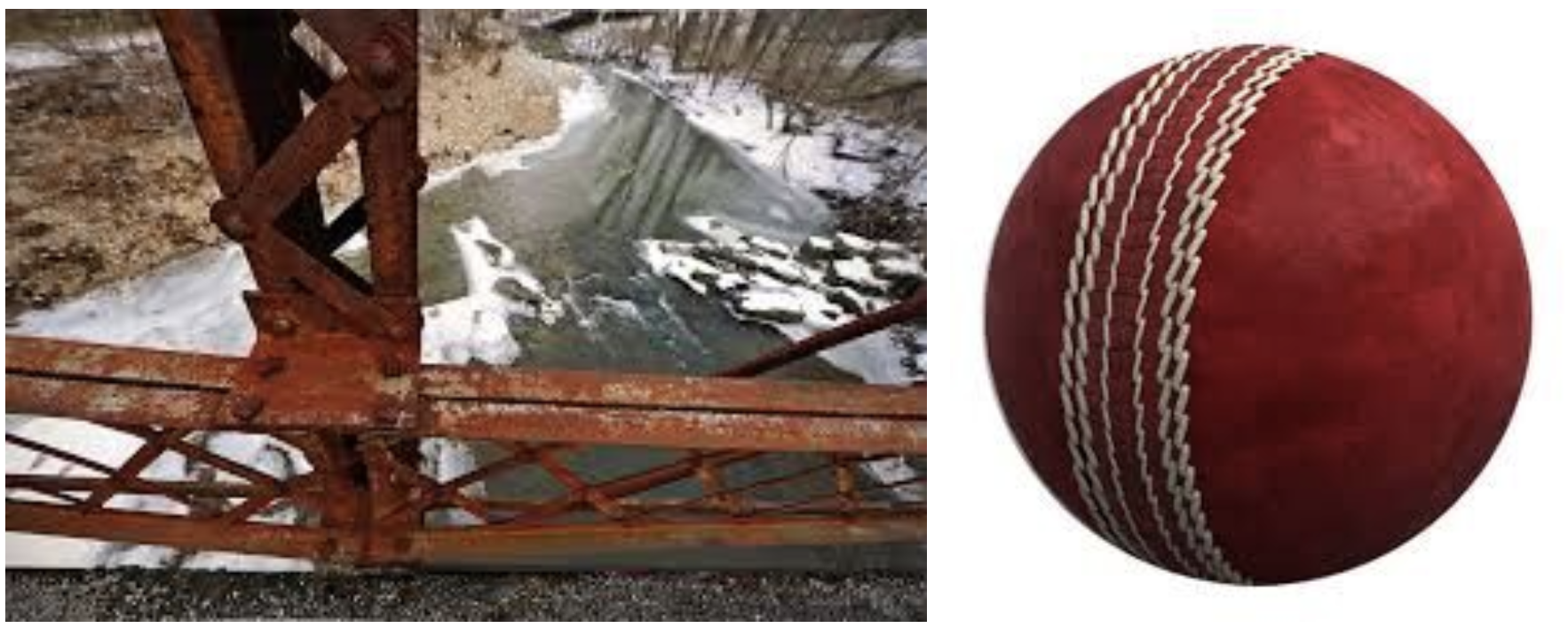
Detecting corrosion and rust manually can be extremely time and effort intensive, and even in some cases dangerous. Also, there are problems in the consistency of estimates – the defects identified vary by the skill of inspector.  Ship hull inspection, bridge inspection are some common scenarios where corrosion detection is of critical importance. The manual process of inspection is partly eliminated by having robotic arms or drones taking pictures of components from various angles, and then having an inspector go through these images to determine a rusted component, that needs repair. Even this process can be quite tedious and costly, as engineers have to go through many such images for hours together, to determine the condition of the component. While traditional computer vision techniques have been used with limited success, in the past, in detecting corrosion from images, the advent of Deep Learning has opened up a whole new possibility, which could lead to accurate detection of corrosion with little or no manual intervention.

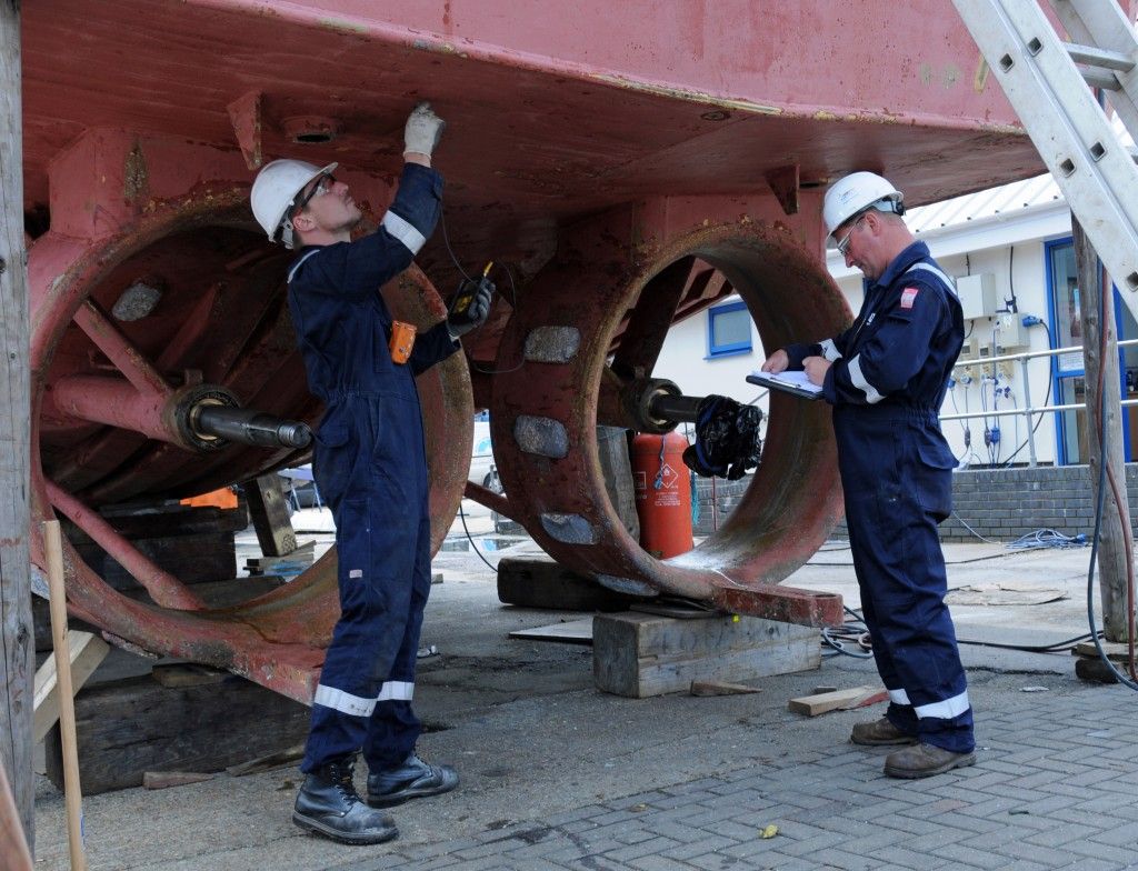
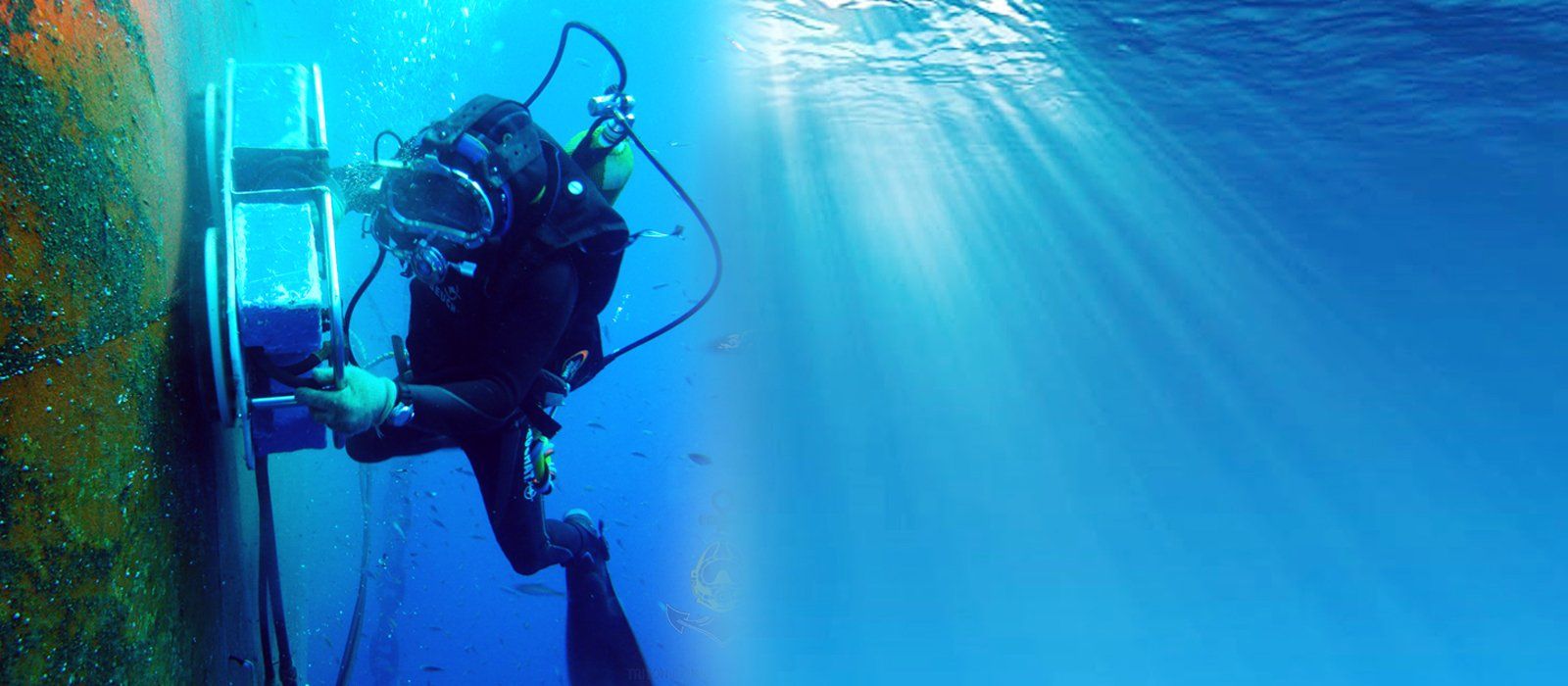
Let’s look at ship hull inspection, one of the common applications of corrosion detection. Detection of corrosion here is extremely important and done manually by experts who inspect the hull and mark the areas to be treated or repaired. It is a time-consuming process due to the large dimensions of the ship (sometimes upwards of 600,000 square meters), and the accuracy is usually poor due to limited visibility. Besides, the surveys are often performed in hazardous environments and the operational conditions turn out to be extreme for human operation. Not to mention the total expenses can be as high as one million euros per ship per inspection cycle!

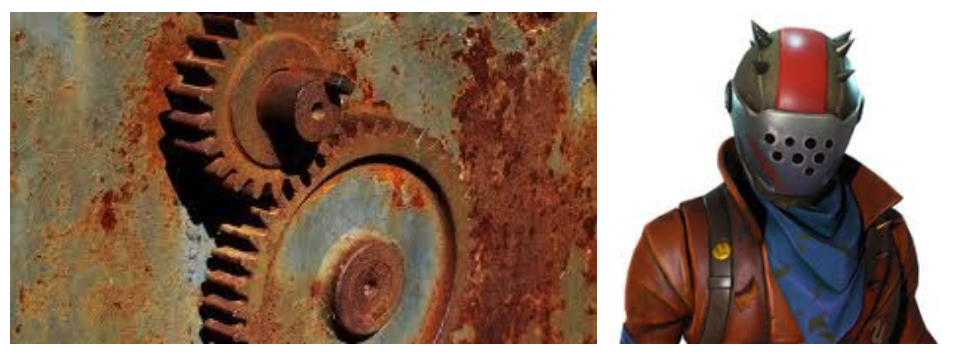
Now let’s look at how we can use computer vision to alleviate this problem. A simple computer vision technique, like applying red filter and classifying as rust based on a threshold level of red, can be a quick way to identify rust. But this naive approach has its limitations, as it detects rust on the presence of a certain color (which can be a painted surface as well). To be more accurate, a more complex feature-based model will be needed, which will consider the texture features as well. Applying this to rust detection can be quite challenging since rust does not have a well-defined shape or color. To be successful with traditional Computer Vision techniques, one needs to bring in complex segmentation, classification and feature measures. This is where Deep Learning comes in. The fundamental aspect of Deep Learning is that it learns complex features on its own, without someone specifying the features explicitly. This means, using a good Deep Learning model might enable us to extract the features of rust automatically, as we train the model with rusted components.

Deep Learning techniques have been known to extract texture based features very effectively. Moreover, we now have a library of pre-trained models (ImageNet-trained CNNs in particular) available as part of open source repositories. The spatial feature hierarchy learned by the pre-trained model effectively acts as a generic model, and hence its features can be used for a different computer vision problem that might involve a completely different classification. Such portability of learned features across different problems is a key advantage of deep learning and it makes deep learning very effective for a small-data scenario. This technique of using pre-trained CNNs on a smaller dataset is known as ‘Transfer Learning’ and is one of the main drivers of the success of deep learning techniques in solving business problems.

We tackle this problem as a two-step process. First, we use Deep Learning with pre-trained models, to do binary classification of images - those having 'rust' and those with 'no rust'. To our surprise, this works very well.  Once we identify the image as having rust, we develop a deep learning model to draw a bounding box around the rust, using TensorFlow Object Detection API.

Image classification of rust via Transfer-Learning

For the first step of Image classification (rust and norust), we use the pre-trained VGG16 model that Keras provides out-of-the-box via a simple API. Since we are applying transfer-learning, let’s freeze the convolutional base from this pre-trained model and train only the last fully connected layers.

The results are pretty amazing! We get an accuracy of 87%, without any major tinkering with the hyper-parameters or trying out different pre-trained models. Amazing baseline, isn’t it?

Setup

You can run the code below on FloydHub by clicking on the below button:

Alternatively, create a new FloydHub account (if you didn’t have one yet),  create a Project, and startup your FloydHub workspace. Select CPU with TensorFlow 1.12 (should be fine for this task). A FloydHub workspace is an interactive Jupyter Lab environment, that allows you to work with Jupyter notebooks, python scripts and much more. Once the workspace is up and running, open up a Terminal prompt from File - > New - > Terminal and clone my GitHub repo in your workspace (if you are working from your local machine you can clone my repo as well):

git clone https://github.com/anirbankonar123/CorrosionDetector

Now, run the notebook : rust_det-using-a-pretrained-convnet-VGG16.ipynb, step by step.

If you are running on your own environment, we assume you have Anaconda IDE with python 3.6 installed. You need to install TensorFlow and Keras.

# Run this only on your machine
pip install tensorflow==1.12.2  # (or tensorflow-gpu, if you are using a GPU system)
pip install keras==2.2.4

As sanity check, let’s print the version of Keras & TensorFlow(default backend):

import keras
import tensorflow as tf
print('Keras version:', keras.__version__)  # it should be 2.2.4
print('TensorFlow version:', tf.__version__)  # it should be 1.12.2

Data preparation

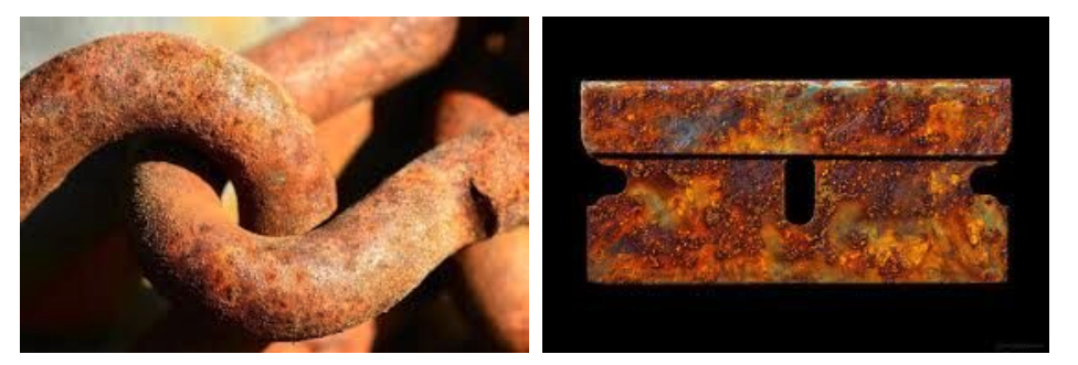
The first step in any Deep Learning process, as usual, is gathering labeled data and dividing up the data into train, test and validation sets. Here comes Google to our help. We simply search ‘rust Images’ on google, and download them. It’s better done manually, to select the good resolution images. The download folder in the Github repo contains all the downloaded images, in sub-folders rust and norust.

The next step is dividing up the data into train set, validation set, and test set. This is accomplished by creating separate folders for train, validation, and test each having sub-folders – rust and norust. Now we can iterate through the downloaded images and copy these into the train, validation, and test folders, following a pattern like label.index.file_extension, e.g: rust.0.jpg, rust.1.jpg, norust.0.jpg, norust.1.jpg.

Here’s the train-val-test split (80-10-10) we use:

• train: 70 rust and 60 no-rust images
• validation: 6 rust and 6 no-rust
• test: 6 rust and 9 no-rust images

The directory structure looks like this, under the base folder( rustnorust_b).

# Type this command under the rustnorust_b folder
$ tree -L 2
.
├── test
│   ├── norust
│   └── rust
├── train
│   ├── norust
│   └── rust
└── validation
    ├── norust
    └── rust

Note that this is a proof of concept to demonstrate the technique. We expect in a professional environment, a strong data collection process to create a dataset able to more accurately represent the underlying data distribution that we want to learn. The code to prepare the images is available in this notebook: rust_det-using-a-pretrained-convnet-VGG16.ipynb

Training images

Since we have just a few images, data augmentation is a necessary technique to train our Deep Learning model. Keras comes to our rescue here. It provides a terrific API (Keras ImageDataGenerator) to generate more images by rotating, shifting, zooming on the images. Please note that validation and test images are not augmented (reference:  Deep Learning with Python: Francois Chollet, Ch 5, Listing 5.21). All images are scaled by dividing the pixels intensities by 255. Feature scaling is a normal practice in the data preparation step.

Augmenting validation or test images will only inflate or deflate the accuracy measure. For example, if the original image is classified correctly, the resulting 100 images from augmentation of this image will also be classified correctly. It could be the other way as well!

train_datagen = ImageDataGenerator(
      rescale=1./255,
      rotation_range=30,
      width_shift_range=0.2,
      height_shift_range=0.2,
      shear_range=0.2,
      zoom_range=0.2,
      horizontal_flip=True,
      fill_mode='nearest')

test_datagen = ImageDataGenerator(rescale=1./255)

train_generator = train_datagen.flow_from_directory(
        train_dir,
        target_size=(150, 150),
        batch_size=4,
        class_mode='binary')

validation_generator = test_datagen.flow_from_directory(
        validation_dir,
        target_size=(150, 150),
        batch_size=16,
        class_mode='binary')

Model creation and training

Once we have prepared our training data, we can create our Convolutional Neural Network model to train on these images. As a first step, we import the pre-trained VGG16, with weights from the ImageNet trained model. The include_top = False implies we do not include the last fully connected layers in the model, the reason being, as mentioned above, we are applying transfer-learning.

conv_base = VGG16(weights='imagenet',include_top=False,input_shape=(150, 150, 3))

This model has 14.7 M parameters! Curious about what it looks like?! You can print it out with this statement: conv_base.summary().

It’s time to create our Neural Network model, using the convolutional base (pre-trained) and add the dense layers on top for our training. Note that this statement conv_base.trainable = False makes sure to freeze the convolutional base of the model. By doing this, the first part of the model will act as a feature extractor and the last layers we have just added at the top will classify the images according to our task.

model = models.Sequential()
model.add(conv_base)
model.add(layers.Flatten())
model.add(layers.Dense(256, activation='relu'))
model.add(layers.Dense(1, activation='sigmoid'))

# Freeze the Convolutional Base
conv_base.trainable = False

Model Summary

The number of trainable parameters in the new model is reduced to 2 M from the original 14.7 M parameters of the full model. This is expected since we freeze the convolutional base (with a series of convolution and pooling layers of the VGG16 model) and train the fully connected layers only.

We use RMSProp optimizer and binary cross-entropy loss (reference:  Deep Learning with Python: Francois Chollet, Ch 5). We train the model for 30 epochs feeding it the output of the ImageDataGenerator, and as you can see in the evaluation step the results are quite amazing!

tensorboard = keras.callbacks.TensorBoard(log_dir='logs/{}'.format(time()))
model.compile(loss='binary_crossentropy',optimizer=optimizers.RMSprop(lr=2e-5),metrics=['acc'])
 
history = model.fit_generator(train_generator,steps_per_epoch=10,epochs=15,validation_data=validation_generator,validation_steps=20,verbose=2,callbacks=[tensorboard])

How do we know how well the model is doing with the validation data? A good approach is to plot the training and validation loss/accuracy with epoch number. The result shows the validation data fits well in the model, and there is no overfitting.

On Floydhub, Tensorboard is enabled by default for all jobs and workspaces, so we can also observe the training via Tensorboard and check the validation accuracy in real-time to see how it is increasing with epochs. Just click the Tensorboard icon at the bottom of the screen, from the FloydHub workspace, and select the CorrosionDetector logs from the left pane.

Model validation

Now comes the all-important step. Exposing our model to images it has not seen before (the test images) and evaluating the model.

test_generator = test_datagen.flow_from_directory(
        test_dir,
        target_size=(150, 150),
        batch_size=4,
        shuffle=False, 
        class_mode='binary')

test_loss, test_acc = model.evaluate_generator(test_generator, steps=10)
print('test acc:', test_acc)

We get an accuracy of 86.1 %. Great! The model is working good on test images. Now let’s do some basic checks. Let’s see for ourselves the prediction generated by the model on a few sample images.

The process is quite easy. We load the test image with target size, as used in the model, convert the image to Numpy array representation and use this to predict the output class of the image (probability >0.5 signifying rust, probability <=0.5 signifying no presence of rust). The result of two sample test images is shown here.

%matplotlib inline
img_path = 'rustnorust_b/test/rust/rust.78.jpg'
# Read the image and resize it
img = image.load_img(img_path, target_size=(150, 150))
plt.imshow(img)
# Convert it to a Numpy array with shape (150, 150, 3)
test_x = image.img_to_array(img)
# Reshape it to (1, 150, 150, 3)
test_x = test_x.reshape((1,) + test_x.shape)
# Normalize the image (we need to do this as we did this same step while training the # model)
test_x = test_x.astype('float32') / 255
rust_prob = model.predict(test_x)

if (rust_prob > 0.5):
    print("This is a rust image")
else:
    print("This is a no rust image")

Output: "This is a rust image"

Output: "This is a no rust image"

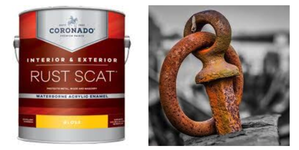
Voilà! it works well. It identifies a reddish brown painted surface as no rust. You can test on your own images. Just click the Upload button from the left pane of your FloydHub workspace, and select an image of your choice. Change the path of the image in the above script and run your prediction (by default all images are uploaded into your home directory: /floyd/home).

Few more tests on images downloaded from the internet

We test our model on random images and run the prediction model, making sure we try to confuse the model with reddish-brown surfaces which are 'no rust' and got pretty good results. We see there are few inaccuracies as well. The readers can explore this further with different training parameters (number of layers, number of neurons), different pre-trained models and check.

Binary classification has few measures of accuracy beyond simple‘Accuracy’. These are precision and recall. Precision is defined by the proportion of predicted rust images which are actually rust(true positives) in the set of all predicted rust images. Recall is the predicted rust images, which are actually rust(true positives) in the set of all genuine rust images. As we can understand Recall is much more important here as we want to detect all rust images. We want it to be 100%. If the Precision is < 100% it means we are labeling a few 'no rust' images as 'rust', which is still fine. We obtain these by running our model on the test data. The Scikit-learn metrics library calculates the binary classification metrics based on the actual label and predicted label.

predictions=model.predict_generator(test_data_generator, steps=test_steps_per_epoch)
val_preds = np.zeros((predictions.shape[0],1))
for i in range(predictions.shape[0]):
    if predictions[i]>0.5:
        val_preds[i] = 1
    else:
        val_preds[i] = 0
val_trues = test_data_generator.classes
labels = test_data_generator.class_indices.keys()
from sklearn.metrics import classification_report
report = classification_report(val_trues, val_preds, target_names=labels)

Classification Report on Test Images

            precision    recall  f1-score   support

     norust       0.89      0.89      0.89         9
       rust       0.83      0.83      0.83         6

avg / total       0.87      0.87      0.87        15

A visual depiction of Confusion Matrix helps understand how good our model is doing in a more intuitive way. As we can see out of 6 true rust images, 5 are classified correctly, and out of 9 true 'no rust' images, 8 are classified correctly in this case.

Finally, there is one other important measure of binary classification - the the ROC-AUC. Let’s check this as well. We use ROC (Receiver Operating Characteristics)-AUC (Area Under The Curve) to check the performance of a binary or multi-class classification. ROC is a probability curve and AUC represents the degree or measure of separability. Basically, it tells us how capable the model is of distinguishing between the ‘rust’ and ‘no rust’ classes. The higher the AUC the better the model is at predicting the classes. For the model to be classified as a good performing model, the AUC should be close to 1. Here’s what we get, the Area under the Curve (AUC) is a healthy 0.85. So we are good here too. Our model is a good baseline at distinguishing rust and no rust images.

To improve the model, please try out with your own images, adding to the training data in the process. Also try out different image classification models available in the Keras API, like the VGG19, ResNet50. Finally try training for more epochs, changing the batch size and using a different optimizer. These are some of the hyperparameters on which you can play to improve your model. For a deeper dive into this topic, please check this detailed article.

Localization and detection of rust

Once we correctly classify a rust image, we go to the next step of localizing and identifying the rusty part in the image by drawing a bounding box on the rust.
We use the TensorFlow Object Detection API, a proven library for this purpose. We only use 40 images for this training all of them being a subset of the images downloaded from the internet. This is because not all the rust images we downloaded are of the form where a bounding box can be drawn over the rusted portion.
The Object detection steps require a bit more attention. There are few dependencies to be installed, environment variables to be set, TFRecords to be generated and fed into the model (normal images don’t work here). So please make sure you do these steps one by one, and do each of them. All the code is in the GitHub repo.

Detecting & Localizing rust with TensorFlow Object Detection API

The steps in a nutshell are:

• Install all dependencies and set environment variables
• Annotate the images using an annotation tool ex: labelImg.  This process is basically drawing boxes around the rust in the image. The labelImg tool automatically creates an XML file that describes the position of the rust in the image. We need to make sure the name of the XML file corresponds to the name of the image exactly
• Split this data into train/test samples
• Convert the XML files into CSV files and then generate TFRecords from these(which is needed by TensorFlow Object Detection API)
• Download the pre-trained model of choice from TensorFlow model zoo and edit the configuration file, based on your setting
• Train the model using the Python script provided
• Export Inference graph (python script provided) from newly trained model, to be used to localize rust on images in real time!
• Evaluate the model using Python script provided

Setup

Start the FloydHub workspace, select GPU with TensorFlow 1.12 (since the training process of Object localization is time consuming).  Selecting a GPU enabled environment is easy in FloydHub, just select GPU from the drop-down while starting your workspace!

Once the workspace is up and running, open up a Terminal prompt from File - > New - > Terminal and do the following setup steps. These setup steps are needed only for the first time.

You can run the entire workspace on FloydHub just by clicking on the below link:

# Important: these setup steps are needed for the first time only
git clone https://github.com/tensorflow/models

# Decomment the following line, if you want to run on the same commit where I tested the code
# cd models && git checkout -q b00783d && cd ..
pip install --user contextlib2
 
#Install Cocoa API :
git clone https://github.com/cocodataset/cocoapi.git
cd cocoapi/PythonAPI
make
cp -r pycocotools /floyd/home/models/research/

# Download and Install Protoc:
wget https://github.com/protocolbuffers/protobuf/releases/download/v3.7.1/protoc-3.7.1-linux-x86_64.zip
cp bin/protoc /usr/local/bin/.
cd models/research 
/usr/local/bin/protoc object_detection/protos/*.proto --python_out=.

# Important: update PYTHONPATH env variable (needed for every restart of workspace):
export PYTHONPATH=$PYTHONPATH:/floyd/home/models/research/:/floyd/home/models/research/slim:/usr/local/bin/

Data preparation

The labeling tool can be used to annotate the images by drawing a box around the rust. Once done, the output is saved as XML file.

# Run this locally
git clone https://github.com/tzutalin/labelImg
python labelImg.py

Using the tool is simple, as shown here. Select the directory where the rust images are present and do Open Dir. This process helps to select the images one by one. Open an image and do Edit – create Bounding Box or just click W. Now, create a bounding box around the rust. Save.

Once it’s saved, the results are stored in XML files. We make sure the XML file has the same name as the image, with the suffix .xml, e.g. rust.0.xml.

Let’s take a look inside the XML file to see what it stores. As we can see it is storing the coordinates of the corners of the bounding box, that we annotated in the image.

<annotation>
<folder>rust</folder>
<filename>rust.30.jpg</filename>
<path>rustnorust_b/train/rust/rust.30.jpg</path>
<source><database>Unknown</database></source>
<size><width>406</width>
<height>340</height>
<depth>3</depth></size>
<segmented>0</segmented>
<object><name>rust</name>
<pose>Unspecified</pose>
<truncated>0</truncated>
<difficult>0</difficult>
<bndbox>
<xmin>73</xmin>
<ymin>7</ymin>
<xmax>359</xmax>
<ymax>339</ymax>
</bndbox>
</object>
</annotation>

As usual, we divide the images into train and test sets and put the image with associated XML in train and test folders, under any suitable directory. In the GitHub repository, this is in  CorrosionDetector/objDet.

Creating TFRecords

We can now create TFRecords. This is the input needed by TensorFlow Object Detection API. The TFRecord format is a simple format for storing a sequence of binary records. The binary data takes up less space on disk, takes less time to copy and can be read much more efficiently from disk, and is particularly useful if the data is being streamed over a network. It provides caching facilities and this helps for datasets that are too large to be stored fully in memory. Only the data that is required at the time (e.g. a batch) is loaded from disk and then processed.

The first step is to convert the XML files saved from the Image annotation process into CSV format. We use the xml_to_csv script for this purpose.

cd models/research/object_detection
# Copy the train and test images into the workspace 
mkdir images
cp -r /floyd/home/CorrosionDetector/objDet/* images/.
cp /floyd/home/CorrosionDetector/xml_to_csv.py .
python xml_to_csv.py

Once this command runs, the train_labels.csv and test_labels.csv should be present in the data directory under models/research/object_detection.

Now we run generate_tfrecord.py to generate TFRecord files from the CSV files. We need to copy the train and test images for the Object Detection into the images folder (under models/research/object_detection). This has been provided in the objDet folder in the GitHub repo.

cp /floyd/home/CorrosionDetector/generate_tfrecord.py .
# Edit the file generate_tfrecord.py, and update the path of the images directory in main method : path = os.path.join(os.getcwd(),'images/train')

python generate_tfrecord.py --csv_input=data/train_labels.csv --output_path=data/train.record

# Edit the file generate_tfrecord.py, and update the path of the images directory in main method : path = os.path.join(os.getcwd(),'images/test')

python generate_tfrecord.py --csv_input=data/test_labels.csv –-output_path=data/test.record

he TFRecord format files( train.record and test.record) should be now present in the data folder. The TFRecords files for this example have been made available in the GitHub repo, as train.record and test.record. This concludes the preparation of training and test data.

Training the Rust Localization Model

There are a number of pre-trained models which can be utilized for this purpose in the TensorFlow Model Zoo. We used the  ssd_mobilenet_v1_coco_11_06_2017 model and trained this for our need. The SSD (Single-shot-detector) is one of the best models for Object Localization.

We download the pre-trained model and unzip the file.

cd models/research/object_detection
wget http://download.tensorflow.org/models/object_detection/ssd_mobilenet_v1_coco_11_06_2017.tar.gz
# Unzip the model file downloaded
tar xvf ssd_mobilenet_v1_coco_11_06_2017.tar.gz

TensorFlow Object Detection API needs to have a certain configuration provided to run effectively. The file ssd_mobilenet_v1_pets.config has been updated and made available in the GitHub repo, to match the configuration based on our needs, providing the path to training data, test data, and label map file prepared in the previous step.

num_classes = 1
train_config: {
  batch_size: 4 # You can play with this hyperparameter
 
tf_record_input_reader {
    input_path: "data/train.record"
  }
  label_map_path: "training/rust_label_map.pbtxt"
 
eval_input_reader: {
  tf_record_input_reader {
    input_path: "data/test.record"
  }
label_map_path: "training/rust_label_map.pbtxt"

Copy the config file and label_map into the proper directory, for the training process to run smoothly.

cd models/research/object_detection
# Copy the TFRecords (train and test) to the data folder (if you have not created it already)
cp /floyd/home/CorrosionDetector/*.record data/.
# Copy the config file and label_map file to the training folder
mkdir training
cp /floyd/home/CorrosionDetector/ssd_mobilenet_v1_pets.config  training/.
cp /floyd/home/CorrosionDetector/rust_label_map.pbtxt training/.

The TensorFlow Object Detection API repository comes with Python scripts to train the model and run the prediction. We use the filetrain.py (from object_detection/legacy). Run the script from the object_detection directory with arguments as shown here. Running the file from the base folder mean the paths will be relative to this folder, and the script will run fine, without any path issues.

cd models/research/object_detection
cp legacy/train.py .
python train.py --logtostderr --train_dir=training/ --pipeline_config_path=training/ssd_mobilenet_v1_pets.config

We can see the loss reducing gradually on the Terminal.

We can follow the progress from TensorBoard, as well.

We can wait till the training completes or if we are a little impatient to try out our new rust localization model, we can take an intermediate checkpoint file. A good rule of thumb is to take a model checkpoint file, once the loss stabilizes and does not reduce much further(check for a value < 3 or between 1 and 3 to get the first insights of training).

The intermediate checkpoint files are stored in models/research/object_detection/training folder and there are three of them in a set, like

model.ckpt-10150.data-0000-of-0001
model.ckpt-10150.index
model.ckpt-10150.meta (the number 10150 will be the step number)

Next step is to export the model into an inference_graph, which can be used for the Rust localization, the final step.

python export_inference_graph.py \
    --input_type image_tensor \
    --pipeline_config_path training/ssd_mobilenet_v1_pets.config \
    --trained_checkpoint_prefix training/model.ckpt-10150 \ #replace this number from your run
    --output_directory rust_inf_graph 

After running this command, the file frozen_inference_graph.pb should be present in the output_directory: rust_inf_graph. This has been provided in the GitHub repo and you can copy this file from GitHub repository to the rust_inf_graph directory, as well.

cd models/research/object_detection
mkdir rust_inf_graph
cp /floyd/home/CorrosionDetector/frozen_inference_graph.pb rust_inf_graph/.

Running the Rust Localization Model

Now open the notebook rust_localization.ipynb from the models/research/object_detection folder. For running this step, you might as well restart the workspace with CPU.

Create a folder test_images under models/research/object_detection and copy a few test images into this folder from objDet/test folder. You can even copy few images from train folder or your own images just to see how the object localization is working.

cd models/research/object_detection
cp /floyd/home/CorrosionDetector/rust_localization.ipynb .
mkdir test_images
cp /floyd/home/CorrosionDetector/objDet/test/*.jpg test_images/.
cp /floyd/home/CorrosionDetector/objDet/train/rust.46.jpg test_images/.

Update the TEST_IMAGE_PATHS in the Cell under Detection and provide the image numbers of your choice, the ones that you want to test the rust localization.
Run the remaining Cells and we can see the rust locations with bounding boxes around them! Even with so few images, the ssd_mobilenet does a pretty decent job of pointing out the rusted locations in the image, and this is not unexpected since ssd_mobilenet uses VGG16 as its base model (which gave us good results in the rust detection).

Evaluation

Evaluation of the model can be done using the script eval.py from the models/research/object_detection/legacy directory.

cd models/research/object_detection
cp legacy/eval.py .
python eval.py --logtostderr --checkpoint_dir=training --eval_dir=eval --pipeline_config_path=training/ssd_mobilenet_v1_pets.config

The output values are not very good in this case, and this was expected since our number of images for this step are just a few(we did not get good quality images from the internet to train the Object detection, as in most of the images there is no specific area where rust can be localized). We expect in a production environment good quality images will be available, to train the Object Detection API.

Average Precision  (AP) @[ IoU=0.50:0.95 | area=   all | maxDets=100 ] = 0.068
Average Precision  (AP) @[ IoU=0.50      | area=   all | maxDets=100 ] = 0.183
Average Precision  (AP) @[ IoU=0.75      | area=   all | maxDets=100 ] = 0.028
Average Recall     (AR) @[ IoU=0.50:0.95 | area=   all | maxDets=  1 ] = 0.075
Average Recall     (AR) @[ IoU=0.50:0.95 | area=   all | maxDets= 10 ] = 0.169
Average Recall     (AR) @[ IoU=0.50:0.95 | area=medium | maxDets=100 ] = 0.100

Similarly to the binary classification task of above, the model can be improved by trying the more updated models as they come in the TensorFlow Model Zoo, using more good quality training images, training for longer time etc. Even in this case, you can perform an hyperparameters search to improve your model.

Conclusion

The article shows how the Image Classification and Object Detection API together can do a great job of inspection - in this case, rusty components. The same can be extended to different scenarios. For example, inspection on manufacturing shop floor for a defective weld and locating faulty welds. As the system is used it gets more images to train on the performance gets better with time. This is something Prof Andrew Ng calls the ‘Virtuous Cycle of AI’ in his AI Transformation Playbook.

The result can be seen as saving in inspection cost, better quality products, and detection of a defect at an early stage thereby reducing rework. In actual production, the trained model can be integrated with an IoT system leading to automatic segregation of good and defective parts. Such AI enabled intelligent Inspection systems are going to become a norm in near future and Deep Learning is going to play an integral role in these. Many such applications are possible with the same process outlined here. Would love to know how you used this process in your domain, or any improvements you did on the model, or any feedback. My contact information is given at the bottom.

Thanks to Cognizant Digital Business, Artificial Intelligence & Analytics, for creating this Proof of Concept idea in the area of Computer Vision. Thanks to the great course content on Coursera and Deeplearning.ai (you can find the review of these courses here) explaining the basic concepts of Convolutional Neural Networks, Transfer Learning and Image augmentation.

FloydHub Call for AI writers

Want to write amazing articles like Anirban and play your role in the long road to Artificial General Intelligence? We are looking for passionate writers, to build the world's best blog for practical applications of groundbreaking A.I. techniques. FloydHub has a large reach within the AI community and with your help, we can inspire the next wave of AI. Apply now and join the crew!

About Anirban Konar
Anirban is a practicing Data Scientist, working at Cognizant Technology Solutions, Kolkata. He takes a keen interest in the latest developments in AI. He keeps himself updated by doing online courses, reading blogs, writing code, and interacting on social media. Anirban is a FloydHub AI Writer. You can connect with Anirban via Twitter, LinkedIn, Facebook and GitHub.