Gated Recurrent Unit (GRU) With PyTorch
The Gated Recurrent Unit (GRU) is the newer version of the more popular LSTM. Let's unveil this network and explore the differences between these 2 siblings.


Have you heard of GRUs?
The Gated Recurrent Unit (GRU) is the younger sibling of the more popular Long Short-Term Memory (LSTM) network, and also a type of Recurrent Neural Network (RNN). Just like its sibling, GRUs are able to effectively retain long-term dependencies in sequential data. And additionally, they can address the “short-term memory” issue plaguing vanilla RNNs.
Considering the legacy of Recurrent architectures in sequence modelling and predictions, the GRU is on track to outshine its elder sibling due to its superior speed while achieving similar accuracy and effectiveness.
In this article, we’ll walk through the concepts behind GRUs and compare the mechanisms of GRUs against LSTMs. We’ll also explore the performance differences in these two RNN variants. If you are unfamiliar with RNNs or LSTMs, you can have a look through my previous posts covering those topics:
What are GRUs?
A Gated Recurrent Unit (GRU), as its name suggests, is a variant of the RNN architecture, and uses gating mechanisms to control and manage the flow of information between cells in the neural network. GRUs were introduced only in 2014 by Cho, et al. and can be considered a relatively new architecture, especially when compared to the widely-adopted LSTM, which was proposed in 1997 by Sepp Hochreiter and Jürgen Schmidhuber.
The structure of the GRU allows it to adaptively capture dependencies from large sequences of data without discarding information from earlier parts of the sequence. This is achieved through its gating units, similar to the ones in LSTMs, which solve the vanishing/exploding gradient problem of traditional RNNs. These gates are responsible for regulating the information to be kept or discarded at each time step. We’ll dive into the specifics of how these gates work and how they overcome the above issues later in this article.
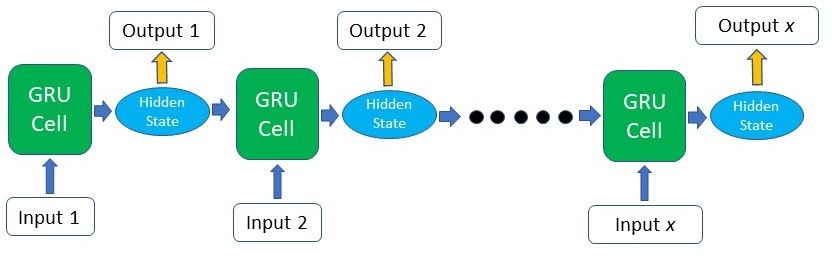
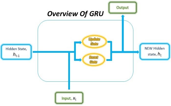
Other than its internal gating mechanisms, the GRU functions just like an RNN, where sequential input data is consumed by the GRU cell at each time step along with the memory, or otherwise known as the hidden state. The hidden state is then re-fed into the RNN cell together with the next input data in the sequence. This process continues like a relay system, producing the desired output.
But How Does It Really Work? Inner Workings of the GRU
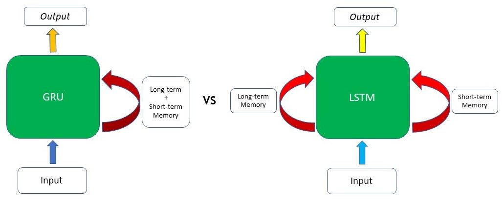
The ability of the GRU to hold on to long-term dependencies or memory stems from the computations within the GRU cell to produce the hidden state. While LSTMs have two different states passed between the cells — the cell state and hidden state, which carry the long and short-term memory, respectively — GRUs only have one hidden state transferred between time steps. This hidden state is able to hold both the long-term and short-term dependencies at the same time due to the gating mechanisms and computations that the hidden state and input data go through.
The GRU cell contains only two gates: the Update gate and the Reset gate. Just like the gates in LSTMs, these gates in the GRU are trained to selectively filter out any irrelevant information while keeping what’s useful. These gates are essentially vectors containing values between 0 to 1 which will be multiplied with the input data and/or hidden state. A 0 value in the gate vectors indicates that the corresponding data in the input or hidden state is unimportant and will, therefore, return as a zero. On the other hand, a 1 value in the gate vector means that the corresponding data is important and will be used.
I’ll be using the terms gate and vector interchangeably for the rest of this article, as they refer to the same thing.
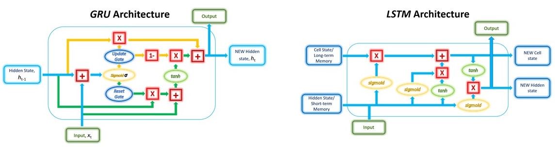
The structure of a GRU unit is shown below.
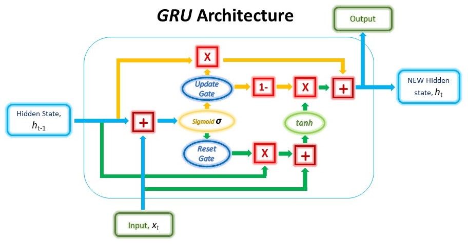
While the structure may look rather complicated due to the large number of connections, the mechanism behind it can be broken down into three main steps.
Reset Gate
In the first step, we’ll be creating the Reset gate. This gate is derived and calculated using both the hidden state from the previous time step and the input data at the current time step.
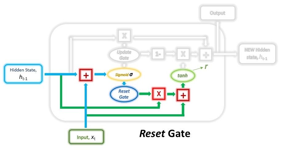
Mathematically, this is achieved by multiplying the previous hidden state and current input with their respective weights and summing them before passing the sum through a sigmoid function. The sigmoid function will transform the values to fall between 0 and 1, allowing the gate to filter between the less-important and more-important information in the subsequent steps.
$$gate_{reset} = \sigma(W_{input_{reset}} \cdot x_t + W_{hidden_{reset}} \cdot h_{t-1})$$
When the entire network is trained through back-propagation, the weights in the equation will be updated such that the vector will learn to retain only the useful features.
The previous hidden state will first be multiplied by a trainable weight and will then undergo an element-wise multiplication (Hadamard product) with the reset vector. This operation will decide which information is to be kept from the previous time steps together with the new inputs. At the same time, the current input will also be multiplied by a trainable weight before being summed with the product of the reset vector and previous hidden state above. Lastly, a non-linear activation tanh function will be applied to the final result to obtain r in the equation below.
$$r = tanh(gate_{reset} \odot (W_{h_1} \cdot h_{t-1}) + W_{x_1} \cdot x_t)$$
Update Gate
Next, we’ll have to create the Update gate. Just like the Reset gate, the gate is computed using the previous hidden state and current input data.
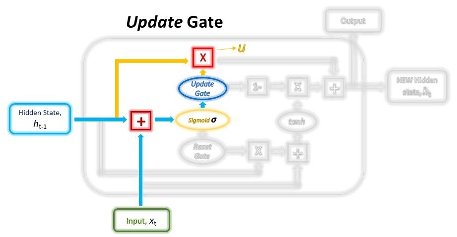
Both the Update and Reset gate vectors are created using the same formula, but, the weights multiplied with the input and hidden state are unique to each gate, which means that the final vectors for each gate are different. This allows the gates to serve their specific purposes.
$$gate_{update} = \sigma(W_{input_{update}} \cdot x_t + W_{hidden_{update}} \cdot h_{t-1})$$
The Update vector will then undergo element-wise multiplication with the previous hidden state to obtain u in our equation below, which will be used to compute our final output later.
$$u = gate_{update} \odot h_{t-1}$$
The Update vector will also be used in another operation later when obtaining our final output. The purpose of the Update gate here is to help the model determine how much of the past information stored in the previous hidden state needs to be retained for the future.
Combining the outputs
In the last step, we will be reusing the Update gate and obtaining the updated hidden state.
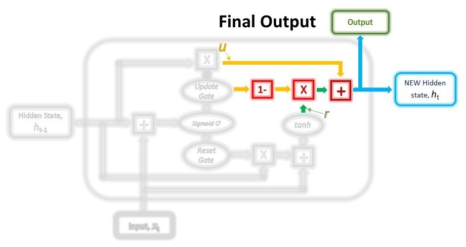
This time, we will be taking the element-wise inverse version of the same Update vector (1 - Update gate) and doing an element-wise multiplication with our output from the Reset gate, r. The purpose of this operation is for the Update gate to determine what portion of the new information should be stored in the hidden state.
Lastly, the result from the above operations will be summed with our output from the Update gate in the previous step, u. This will give us our new and updated hidden state.
$$h_t = r \odot (1-gate_{update}) + u$$
We can use this new hidden state as our output for that time step as well by passing it through a linear activation layer.
Solving the Vanishing / Exploding Gradient Problem
We’ve seen the gates in action. We know how they transform our data. Now let’s review their overall role in managing the network’s memory and talk about how they solve the vanishing/exploding gradient problem.
As we’ve seen in the mechanisms above, the Reset gate is responsible for deciding which portions of the previous hidden state are to be combined with the current input to propose a new hidden state.
And the Update gate is responsible for determining how much of the previous hidden state is to be retained and what portion of the new proposed hidden state (derived from the Reset gate) is to be added to the final hidden state. When the Update gate is first multiplied with the previous hidden state, the network is picking which parts of the previous hidden state it is going to keep in its memory while discarding the rest. Subsequently, it is patching up the missing parts of information when it uses the inverse of the Update gate to filter the proposed new hidden state from the Reset gate.
This allows the network to retain long-term dependencies. The Update gate can choose to retain most of the previous memories in the hidden state if the Update vector values are close to 1 without re-computing or changing the entire hidden state.
The vanishing/exploding gradient problem occurs during back-propagation when training the RNN, especially if the RNN is processing long sequences or has multiple layers. The error gradient calculated during training is used to update the network’s weight in the right direction and by the right magnitude. However, this gradient is calculated with the chain rule, starting from the end of the network. Therefore, during back-propagation, the gradients will continuously undergo matrix multiplications and either shrink (vanish) or blow up (explode) exponentially for long sequences. Having a gradient that is too small means the model won’t update its weights effectively, whereas extremely large gradients cause the model to be unstable.
The gates in the LSTM and GRUs help to solve this problem because of the additive component of the Update gates. While traditional RNNs always replace the entire content of the hidden state at each time step, LSTMs and GRUs keep most of the existing hidden state while adding new content on top of it. This allows the error gradients to be back-propagated without vanishing or exploding too quickly due to the addition operations.
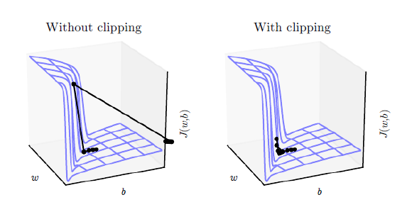
While LSTMs and GRUs are the most widely-used fixes to the above problem, another solution to the problem of exploding gradients is gradient clipping. Clipping sets a defined threshold value on the gradients, which means that even if a gradient increases beyond the predefined value during training, its value will still be limited to the set threshold. This way, the direction of the gradient remains unaffected and only the magnitude of the gradient is changed.
GRU vs LSTM
We’ve got the mechanics of GRUs down. But how does it compare to its older (and more popular) sibling, LSTMs?
Well, both were created to solve the vanishing/exploding gradient problem that the standard RNN faces, and both of these RNN variants utilise gating mechanisms to control the flow of long-term and short-term dependencies within the network.
But how are they different?
- Structural Differences
While both GRUs and LSTMs contain gates, the main difference between these two structures lies in the number of gates and their specific roles. The role of the Update gate in the GRU is very similar to the Input and Forget gates in the LSTM. However, the control of new memory content added to the network differs between these two.
In the LSTM, while the Forget gate determines which part of the previous cell state to retain, the Input gate determines the amount of new memory to be added. These two gates are independent of each other, meaning that the amount of new information added through the Input gate is completely independent of the information retained through the Forget gate.
As for the GRU, the Update gate is responsible for determining which information from the previous memory to retain and is also responsible for controlling the new memory to be added. This means that the retention of previous memory and addition of new information to the memory in the GRU is NOT independent.
Another key difference between the structures is the lack of the cell state in the GRU, as mentioned earlier. While the LSTM stores its longer-term dependencies in the cell state and short-term memory in the hidden state, the GRU stores both in a single hidden state. However, in terms of effectiveness in retaining long-term information, both architectures have been proven to achieve this goal effectively.
2. Speed Differences
GRUs are faster to train as compared to LSTMs due to the fewer number of weights and parameters to update during training. This can be attributed to the fewer number of gates in the GRU cell (two gates) as compared to the LSTM’s three gates.
In the code walkthrough further down in this article, we’ll be directly comparing the speed of training an LSTM against a GRU on the exact same task.
3. Performance Evaluations
The accuracy of a model, whether it is measured by the margin of error or proportion of correct classifications, is usually the main factor when deciding which type of model to use for a task. Both GRUs and LSTMs are variants of RNNS and can be plugged in interchangeably to achieve similar results.
Project: Time-series Prediction with GRU and LSTM
We’ve learnt about the theoretical concepts behind the GRU. Now it’s time to put that learning to work.
We’ll be implementing a GRU model in code. To further our GRU-LSTM comparison, we’ll also be using an LSTM model to complete the same task. We’ll evaluate the performance of both models on a few metrics. The dataset that we will be using is the Hourly Energy Consumption dataset, which can be found on Kaggle. The dataset contains power consumption data across different regions around the United States recorded on an hourly basis.
You can run the code implementation in this article on FloydHub, using their GPUs on the cloud, by clicking the following link and using the main.ipynb notebook:

This will speed up the training process significantly. Alternatively, you can visit the GitHub repository specifically.
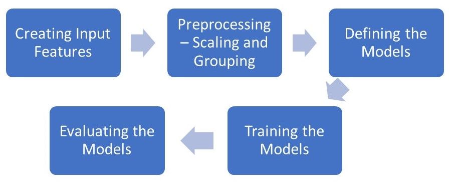
The goal of this implementation is to create a model that can accurately predict the energy usage in the next hour given historical usage data. We will be using both the GRU and LSTM model to train on a set of historical data and evaluate both models on an unseen test set. To do so, we’ll start with feature selection and data pre-processing, followed by defining, training, and eventually evaluating the models.
This will be the process flow of our project.
We will be using the PyTorch library to implement both types of models along with other common Python libraries used in data analytics.
import os
import time

import numpy as np
import pandas as pd
import matplotlib.pyplot as plt

import torch
import torch.nn as nn
from torch.utils.data import TensorDataset, DataLoader

from tqdm import tqdm_notebook
from sklearn.preprocessing import MinMaxScaler

# Define data root directory
data_dir = "./data/"
# Visualise how our data looks
pd.read_csv(data_dir + 'AEP_hourly.csv').head()
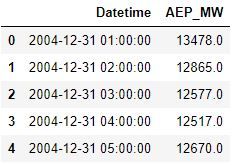
We have a total of 12 .csv files containing hourly energy trend data of the above format ('est_hourly.paruqet' and 'pjm_hourly_est.csv' are not used). In our next step, we will be reading these files and pre-processing these data in this order:
- Get the time data of each individual time step and generalize them
- Hour of the day i.e., 0 - 23
- Day of the week i.e,. 1 - 7
- Month i.e., 1 - 12
- Day of the year i.e., 1 - 365
- Scale the data to values between 0 and 1
- Algorithms tend to perform better or converge faster when features are on a relatively similar scale and/or close to normally distributed
- Scaling preserves the shape of the original distribution and doesn't reduce the importance of outliers
- Group the data into sequences to be used as inputs to the model and store their corresponding labels
- The sequence length or look back period is the number of data points in history that the model will use to make the prediction
- The label will be the next data point in time after the last one in the input sequence
- Split the inputs and labels into training and test sets
# The scaler objects will be stored in this dictionary so that our output test data from the model can be re-scaled during evaluation
label_scalers = {}

train_x = []
test_x = {}
test_y = {}

for file in tqdm_notebook(os.listdir(data_dir)):
    # Skipping the files we're not using
    if file[-4:] != ".csv" or file == "pjm_hourly_est.csv":
        continue

    # Store csv file in a Pandas DataFrame
    df = pd.read_csv('{}/{}'.format(data_dir, file), parse_dates=[0])
    # Processing the time data into suitable input formats
    df['hour'] = df.apply(lambda x: x['Datetime'].hour,axis=1)
    df['dayofweek'] = df.apply(lambda x: x['Datetime'].dayofweek,axis=1)
    df['month'] = df.apply(lambda x: x['Datetime'].month,axis=1)
    df['dayofyear'] = df.apply(lambda x: x['Datetime'].dayofyear,axis=1)
    df = df.sort_values("Datetime").drop("Datetime",axis=1)

    # Scaling the input data
    sc = MinMaxScaler()
    label_sc = MinMaxScaler()
    data = sc.fit_transform(df.values)
    # Obtaining the Scale for the labels(usage data) so that output can be re-scaled to actual value during evaluation
    label_sc.fit(df.iloc[:,0].values.reshape(-1,1))
    label_scalers[file] = label_sc

    # Define lookback period and split inputs/labels
    lookback = 90
    inputs = np.zeros((len(data)-lookback,lookback,df.shape[1]))
    labels = np.zeros(len(data)-lookback)

    for i in range(lookback, len(data)):
        inputs[i-lookback] = data[i-lookback:i]
        labels[i-lookback] = data[i,0]
    inputs = inputs.reshape(-1,lookback,df.shape[1])
    labels = labels.reshape(-1,1)

    # Split data into train/test portions and combining all data from different files into a single array
    test_portion = int(0.1*len(inputs))
    if len(train_x) == 0:
        train_x = inputs[:-test_portion]
        train_y = labels[:-test_portion]
    else:
        train_x = np.concatenate((train_x,inputs[:-test_portion]))
        train_y = np.concatenate((train_y,labels[:-test_portion]))
    test_x[file] = (inputs[-test_portion:])
    test_y[file] = (labels[-test_portion:])
We have a total of 980,185 sequences of training data.
To improve the speed of our training, we can process the data in batches so that the model doesn’t need to update its weights as frequently. The Torch Dataset and DataLoader classes are useful for splitting our data into batches and shuffling them.
batch_size = 1024
train_data = TensorDataset(torch.from_numpy(train_x), torch.from_numpy(train_y))
train_loader = DataLoader(train_data, shuffle=True, batch_size=batch_size, drop_last=True)
We can also check if we have any GPUs to speed up our training time. If you’re using FloydHub with GPU to run this code, the training time will be significantly reduced.
# torch.cuda.is_available() checks and returns a Boolean True if a GPU is available, else it'll return False
is_cuda = torch.cuda.is_available()

# If we have a GPU available, we'll set our device to GPU. We'll use this device variable later in our code.
if is_cuda:
    device = torch.device("cuda")
else:
    device = torch.device("cpu")
Next, we'll be defining the structure of the GRU and LSTM models. Both models have the same structure, with the only difference being the recurrent layer (GRU/LSTM) and the initializing of the hidden state. The hidden state for the LSTM is a tuple containing both the cell state and the hidden state, whereas the GRU only has a single hidden state.
class GRUNet(nn.Module):
    def __init__(self, input_dim, hidden_dim, output_dim, n_layers, drop_prob=0.2):
        super(GRUNet, self).__init__()
        self.hidden_dim = hidden_dim
        self.n_layers = n_layers

        self.gru = nn.GRU(input_dim, hidden_dim, n_layers, batch_first=True, dropout=drop_prob)
        self.fc = nn.Linear(hidden_dim, output_dim)
        self.relu = nn.ReLU()

    def forward(self, x, h):
        out, h = self.gru(x, h)
        out = self.fc(self.relu(out[:,-1]))
        return out, h

    def init_hidden(self, batch_size):
        weight = next(self.parameters()).data
        hidden = weight.new(self.n_layers, batch_size, self.hidden_dim).zero_().to(device)
        return hidden

class LSTMNet(nn.Module):
    def __init__(self, input_dim, hidden_dim, output_dim, n_layers, drop_prob=0.2):
        super(LSTMNet, self).__init__()
        self.hidden_dim = hidden_dim
        self.n_layers = n_layers

        self.lstm = nn.LSTM(input_dim, hidden_dim, n_layers, batch_first=True, dropout=drop_prob)
        self.fc = nn.Linear(hidden_dim, output_dim)
        self.relu = nn.ReLU()

    def forward(self, x, h):
        out, h = self.lstm(x, h)
        out = self.fc(self.relu(out[:,-1]))
        return out, h

    def init_hidden(self, batch_size):
        weight = next(self.parameters()).data
        hidden = (weight.new(self.n_layers, batch_size, self.hidden_dim).zero_().to(device),
                  weight.new(self.n_layers, batch_size, self.hidden_dim).zero_().to(device))
        return hidden
The training process is defined in a function below so that we can reproduce it for both models. Both models will have the same number of dimensions in the hidden state and layers, trained over the same number of epochs and learning rate, and trained and tested on the exact same set of data.
For the purpose of comparing the performance of both models, we'll be tracking the time it takes for the model to train and eventually comparing the final accuracy of both models on the test set. For our accuracy measure, we'll use Symmetric Mean Absolute Percentage Error (sMAPE) to evaluate the models. sMAPE is the sum of the absolute difference between the predicted and actual values divided by the average of the predicted and actual value, therefore giving a percentage measuring the amount of error.This is the formula for sMAPE:
$$sMAPE = \frac{100%}{n} \sum_{t=1}^n \frac{|F_t - A_t|}{(|F_t + A_t|)/2}$$
def train(train_loader, learn_rate, hidden_dim=256, EPOCHS=5, model_type="GRU"):

    # Setting common hyperparameters
    input_dim = next(iter(train_loader))[0].shape[2]
    output_dim = 1
    n_layers = 2
    # Instantiating the models
    if model_type == "GRU":
        model = GRUNet(input_dim, hidden_dim, output_dim, n_layers)
    else:
        model = LSTMNet(input_dim, hidden_dim, output_dim, n_layers)
    model.to(device)

    # Defining loss function and optimizer
    criterion = nn.MSELoss()
    optimizer = torch.optim.Adam(model.parameters(), lr=learn_rate)

    model.train()
    print("Starting Training of {} model".format(model_type))
    epoch_times = []
    # Start training loop
    for epoch in range(1,EPOCHS+1):
        start_time = time.clock()
        h = model.init_hidden(batch_size)
        avg_loss = 0.
        counter = 0
        for x, label in train_loader:
            counter += 1
            if model_type == "GRU":
                h = h.data
            else:
                h = tuple([e.data for e in h])
            model.zero_grad()

            out, h = model(x.to(device).float(), h)
            loss = criterion(out, label.to(device).float())
            loss.backward()
            optimizer.step()
            avg_loss += loss.item()
            if counter%200 == 0:
                print("Epoch {}......Step: {}/{}....... Average Loss for Epoch: {}".format(epoch, counter, len(train_loader), avg_loss/counter))
        current_time = time.clock()
        print("Epoch {}/{} Done, Total Loss: {}".format(epoch, EPOCHS, avg_loss/len(train_loader)))
        print("Total Time Elapsed: {} seconds".format(str(current_time-start_time)))
        epoch_times.append(current_time-start_time)
    print("Total Training Time: {} seconds".format(str(sum(epoch_times))))
    return model

def evaluate(model, test_x, test_y, label_scalers):
    model.eval()
    outputs = []
    targets = []
    start_time = time.clock()
    for i in test_x.keys():
        inp = torch.from_numpy(np.array(test_x[i]))
        labs = torch.from_numpy(np.array(test_y[i]))
        h = model.init_hidden(inp.shape[0])
        out, h = model(inp.to(device).float(), h)
        outputs.append(label_scalers[i].inverse_transform(out.cpu().detach().numpy()).reshape(-1))
        targets.append(label_scalers[i].inverse_transform(labs.numpy()).reshape(-1))
    print("Evaluation Time: {}".format(str(time.clock()-start_time)))
    sMAPE = 0
    for i in range(len(outputs)):
        sMAPE += np.mean(abs(outputs[i]-targets[i])/(targets[i]+outputs[i])/2)/len(outputs)
    print("sMAPE: {}%".format(sMAPE*100))
    return outputs, targets, sMAPE
lr = 0.001
gru_model = train(train_loader, lr, model_type="GRU")
Lstm_model = train(train_loader, lr, model_type="LSTM")
[Out]: Starting Training of GRU model
       Epoch 1......Step: 200/957....... Average Loss for Epoch: 0.0070570480596506965
       Epoch 1......Step: 400/957....... Average Loss for Epoch: 0.0039001358837413135
       Epoch 1......Step: 600/957....... Average Loss for Epoch: 0.0027501484048358784
       Epoch 1......Step: 800/957....... Average Loss for Epoch: 0.0021489552696584723
       Epoch 1/5 Done, Total Loss: 0.0018450273993545988
       Time Elapsed for Epoch: 78.02232400000003 seconds
        .
        .
        .
       Total Training Time: 390.52727700000037 seconds

       Starting Training of LSTM model
       Epoch 1......Step: 200/957....... Average Loss for Epoch: 0.013630141295143403
        .
        .
        .
       Total Training Time: 462.73371699999984 seconds
As we can see from the training time of both models, our younger sibling has absolutely thrashed the older one in terms of speed. The GRU model is the clear winner on that dimension; it finished five training epochs 72 seconds faster than the LSTM model.
Moving on to measuring the accuracy of both models, we’ll now use our evaluate() function and test dataset.
gru_outputs, targets, gru_sMAPE = evaluate(gru_model, test_x, test_y, label_scalers)
[Out]: Evaluation Time: 1.982479000000012
       sMAPE: 0.28081167222194775%
lstm_outputs, targets, lstm_sMAPE = evaluate(lstm_model, test_x, test_y, label_scalers)
[Out]: Evaluation Time: 2.602886000000126
       sMAPE: 0.27014616762377464%
Ahh. Interesting, right? While the LSTM model may have made smaller errors and edged in front of the GRU model slightly in terms of performance accuracy, the difference is insignificant and thus inconclusive.
Other tests comparing both these models have similarly returned no clear winner as to which is the better architecture overall.
Lastly, let's do some visualisations on random sets of our predicted output vs the actual consumption data.
plt.figure(figsize=(14,10))
plt.subplot(2,2,1)
plt.plot(gru_outputs[0][-100:], "-o", color="g", label="Predicted")
plt.plot(targets[0][-100:], color="b", label="Actual")
plt.ylabel('Energy Consumption (MW)')
plt.legend()

plt.subplot(2,2,2)
plt.plot(gru_outputs[8][-50:], "-o", color="g", label="Predicted")
plt.plot(targets[8][-50:], color="b", label="Actual")
plt.ylabel('Energy Consumption (MW)')
plt.legend()

plt.subplot(2,2,3)
plt.plot(gru_outputs[4][:50], "-o", color="g", label="Predicted")
plt.plot(targets[4][:50], color="b", label="Actual")
plt.ylabel('Energy Consumption (MW)')
plt.legend()

plt.subplot(2,2,4)
plt.plot(lstm_outputs[6][:100], "-o", color="g", label="Predicted")
plt.plot(targets[6][:100], color="b", label="Actual")
plt.ylabel('Energy Consumption (MW)')
plt.legend()
plt.show()
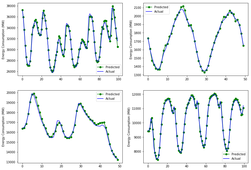
Looks like the models are largely successful in predicting the trends of energy consumption. While they may still get some changes wrong, such as delays in predicting a drop in consumption, the predictions follow very closely to the actual line on the test set. This is due to the nature of energy consumption data and the fact that there are patterns and cyclical changes that the model can account for. Tougher time-series prediction problems such as stock price prediction or sales volume prediction may have data that is largely random or doesn’t have predictable patterns, and in such cases, the accuracy will definitely be lower.
Beyond GRUs
As I mentioned in my LSTM article, RNNs and their variants have been replaced over the years in various NLP tasks and are no longer an NLP standard architecture. Pre-trained transformer models such as Google’s BERT, OpenAI’s GPT and the recently introduced XLNet have produced state-of-the-art benchmarks and results and have introduced transfer learning for downstreamed tasks to NLP.
With that, signing off on all things GRU for now. This piece completes my series of articles covering the basics of RNNs; in future, we’ll be exploring more advanced concepts such as the Attention mechanism, Transformers, and the modern state-of-the-art in NLP. Get hyped.
Special thanks to Alessio for his valuable feedback and advice and the rest of the FloydHub team for providing this amazing platform and allowing me to give back to the deep learning community. Stay awesome!
FloydHub Call for AI writers
Want to write amazing articles like Gabriel and play your role in the long road to Artificial General Intelligence? We are looking for passionate writers, to build the world's best blog for practical applications of groundbreaking A.I. techniques. FloydHub has a large reach within the AI community and with your help, we can inspire the next wave of AI. Apply now and join the crew!
About Gabriel Loye
Gabriel is an Artificial Intelligence enthusiast and web developer. He’s currently exploring various fields of deep learning from Natural Language Processing to Computer Vision. He’s always open to learning new things and implementing or researching on novel ideas and technologies. He’ll soon start his undergraduate studies in Business Analytics at the NUS School of Computing and is currently an intern at Fintech start-up PinAlpha. Gabriel is also a FloydHub AI Writer. You can connect with Gabriel on LinkedIn and GitHub.