Colorizing B&W Photos with Neural Networks

Earlier this year, Amir Avni used neural networks to troll the subreddit /r/Colorization - a community where people colorize historical black and white images manually using Photoshop. They were astonished with Amir’s deep learning bot - what could take up to a month of manual labour could now be done in just a few seconds.

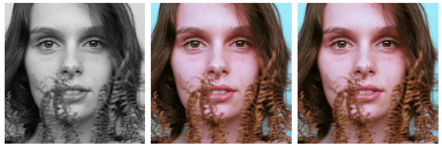
I was fascinated by Amir’s neural network, so I reproduced it and documented the process. First off, let’s look at some of the results/failures from my experiments (scroll to the bottom for the final result).

Today, colorization is done by hand in Photoshop. To appreciate all the hard work behind this process, take a peek at this gorgeous colorization memory lane video. In short, a picture can take up to one month to colorize. It requires extensive research. A face alone needs up to 20 layers of pink, green and blue shades to get it just right.

This article is for beginners. Yet, if you’re new to deep learning terminology, you can read my previous two posts [1][2] and watch Andrej Karpathy’s lecture for more background.

I’ll show you how to build your own colorization neural net in three steps.

The first section breaks down the core logic. We’ll build a bare-bones 40-line neural network as an “Alpha" colorization bot. There’s not a lot of magic in this code snippet - which is helpful so that we can get familiar with the syntax.

The next step is to create a neural network that can generalize - our “Beta” version. We’ll be able to color images the bot has not seen before.

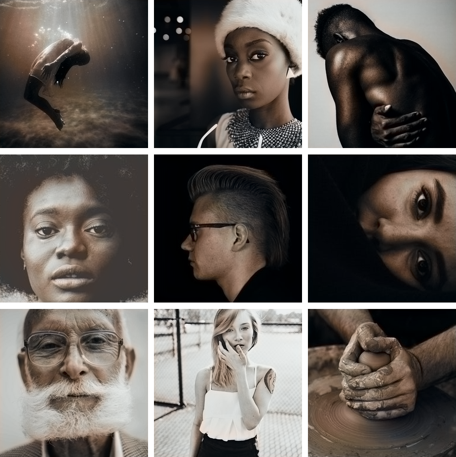
For our “final” version, we’ll combine our neural network with a classifier. We’ll use an Inception Resnet V2 that has been trained on 1.2 million images. To make the coloring pop, we’ll train our neural network on portraits from Unsplash.

If you want to look ahead, here’s a Jupyter Notebook with the Alpha version of our bot. You can also check out the three versions on FloydHub and GitHub, along with code for all the experiments I ran on FloydHub’s cloud GPUs.

Core Logic

In this section, I’ll outline how to render an image, the basics of digital colors, and the main logic for our neural network.

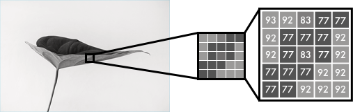
Black and white images can be represented in grids of pixels. Each pixel has a value that corresponds to its brightness. The values span from 0 - 255, from black to white.

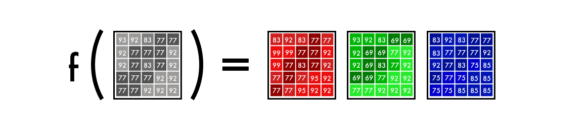
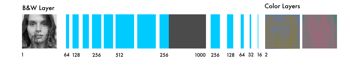
Color images consist of three layers: a red layer, a green layer, and a blue layer. This might be counter-intuitive to you. Imagine splitting a green leaf on a white background into the three channels. Intuitively, you might think that the plant is only present in the green layer.

But, as you see below, the leaf is present in all three channels. The layers not only determine color, but also brightness.

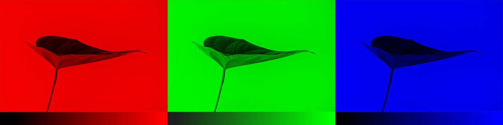
To achieve the color white, for example, you need an equal distribution of all colors. By adding an equal amount of red and blue, it makes the green brighter. Thus, a color image encodes the color and the contrast using three layers:

Just like black and white images, each layer in a color image has a value from 0 - 255. The value 0 means that it has no color in this layer. If the value is 0 for all color channels, then the image pixel is black.

As you may know, a neural network creates a relationship between an input value and output value. To be more precise with our colorization task, the network needs to find the traits that link grayscale images with colored ones.

In sum, we are searching for the features that link a grid of grayscale values to the three color grids.

The Alpha Version

We’ll start by making a simple version of our neural network to color an image of a woman’s face. This way, you can get familiar with the core syntax of our model as we add features to it.

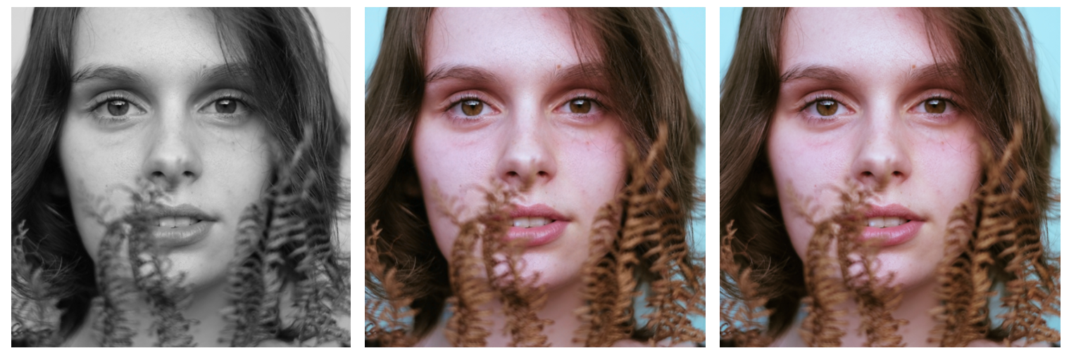
With just 40 lines of code, we can make the following transition. The middle picture is done with our neural network and the picture to the right is the original color photo. The network is trained and tested on the same image - we’ll get back to this during the beta-version.

Color space

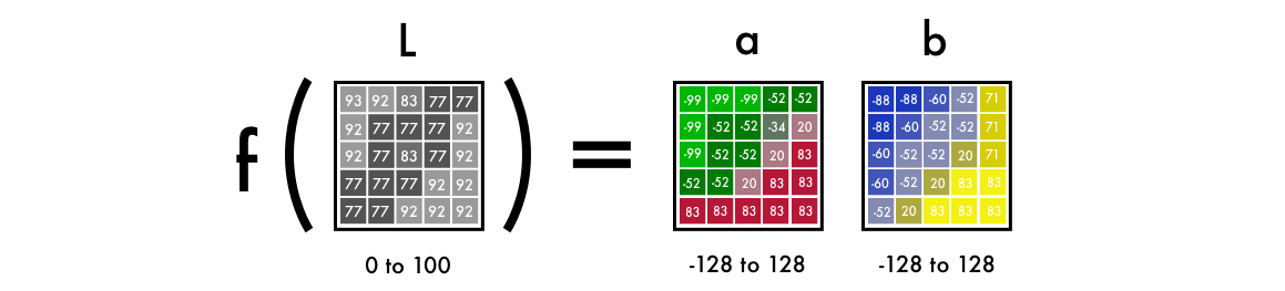
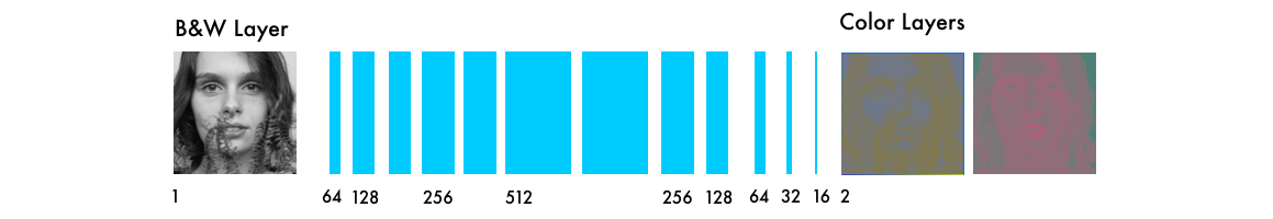
First, we’ll use an algorithm to change the color channels, from RGB to Lab. L stands for lightness, and a and b for the color spectrums green–red and blue–yellow.

As you can see below, a Lab encoded image has one layer for grayscale and have packed three color layers into two. This means that we can use the original grayscale image in our final prediction. Also, we only have to two channels to predict.

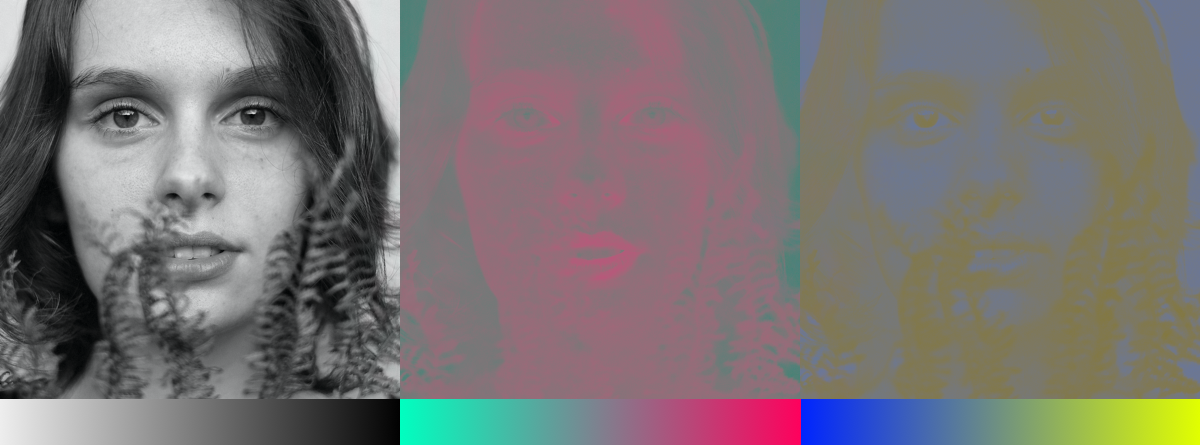
Science fact - 94% of the cells in our eyes determine brightness. That leaves only 6% of our receptors to act as sensors for colors. As you can see in the above image, the grayscale image is a lot sharper than the color layers. This is another reason to keep the grayscale image in our final prediction.

From B&W to color

Our final prediction looks like this. We have a grayscale layer for input, and we want to predict two color layers, the ab in Lab. To create the final color image we’ll include the L/grayscale image we used for the input, thus, creating a Lab image.

To turn one layer into two layers, we use convolutional filters. Think of them as the blue/red filters in 3D glasses. Each filter determines what we see in a picture. They can highlight or remove something to extract information out of the picture. The network can either create a new image from a filter or combine several filters into one image.

For a convolutional neural network, each filter is automatically adjusted to help with the intended outcome. We’ll start by stacking hundreds of filters and narrow them down into two layers, the a and b layers.

Before we get into detail into how it works, let’s run the code.

Deploying the code on FloydHub

If you are new to FloydHub, do their 2-min installation, check my 5-min video tutorial or my step-to-step guide - it’s the best (and easiest) way to train deep learning models on cloud GPUs.

Alpha version

Once FloydHub is installed, use the following commands:

git clone https://github.com/emilwallner/Coloring-greyscale-images-in-Keras

Open the folder and initiate FloydHub.

cd Coloring-greyscale-images-in-Keras/floydhub
floyd init colornet

The FloydHub web dashboard will open in your browser, and you will be prompted to create a new FloydHub project called colornet. Once that's done, go back to your terminal and run the same init command.

floyd init colornet

Okay, let's run our job:

floyd run --data emilwallner/datasets/colornet/2:data --mode jupyter --tensorboard

Some quick notes about our job:

• We mounted a public dataset on FloydHub (which I've already uploaded) at the data directory with --data emilwallner/datasets/colornet/2:data. You can explore and use this dataset (and many other public datasets) by viewing it on FloydHub
• We enabled Tensorboard with --tensorboard
• We ran the job in Jupyter Notebook mode with --mode jupyter
• If you have GPU credit, you can also add the GPU flag --gpu to your command - this will make it ~50x faster

Go to your the Jupyter notebook under the Jobs tab on the FloydHub website, click on the Jupyter Notebook link, and navigate to this file: floydhub/Alpha version/working_floyd_pink_light_full.ipynb. Open it and click shift+enter on all the cells.

Gradually increase the epoch value to get a feel for how the neural network learns.

model.fit(x=X, y=Y, batch_size=1, epochs=1)

Start with an epoch value of 1 and the increase it to 10, 100, 500, 1000 and 3000. The epoch value indicates how many times the neural network learns from the image. You will find the image img_result.png in the main folder once you’ve trained your neural network.

# Get images
image = img_to_array(load_img('woman.png'))
image = np.array(image, dtype=float)

# Import map images into the lab colorspace
X = rgb2lab(1.0/255*image)[:,:,0]
Y = rgb2lab(1.0/255*image)[:,:,1:]
Y = Y / 128
X = X.reshape(1, 400, 400, 1)
Y = Y.reshape(1, 400, 400, 2)

model = Sequential()
model.add(InputLayer(input_shape=(None, None, 1)))

# Building the neural network
model = Sequential()
model.add(InputLayer(input_shape=(None, None, 1)))
model.add(Conv2D(8, (3, 3), activation='relu', padding='same', strides=2))
model.add(Conv2D(8, (3, 3), activation='relu', padding='same'))
model.add(Conv2D(16, (3, 3), activation='relu', padding='same'))
model.add(Conv2D(16, (3, 3), activation='relu', padding='same', strides=2))
model.add(Conv2D(32, (3, 3), activation='relu', padding='same'))
model.add(Conv2D(32, (3, 3), activation='relu', padding='same', strides=2))
model.add(UpSampling2D((2, 2)))
model.add(Conv2D(32, (3, 3), activation='relu', padding='same'))
model.add(UpSampling2D((2, 2)))
model.add(Conv2D(16, (3, 3), activation='relu', padding='same'))
model.add(UpSampling2D((2, 2)))
model.add(Conv2D(2, (3, 3), activation='tanh', padding='same'))

# Finish model
model.compile(optimizer='rmsprop',loss='mse')

#Train the neural network
model.fit(x=X, y=Y, batch_size=1, epochs=3000)
print(model.evaluate(X, Y, batch_size=1))

# Output colorizations
output = model.predict(X)
output = output * 128
canvas = np.zeros((400, 400, 3))
canvas[:,:,0] = X[0][:,:,0]
canvas[:,:,1:] = output[0]
imsave("img_result.png", lab2rgb(cur))
imsave("img_gray_scale.png", rgb2gray(lab2rgb(cur)))

FloydHub command to run this network:

floyd run --data emilwallner/datasets/colornet/2:data --mode jupyter --tensorboard

Technical explanation

To recap, the input is a grid representing a black and white image. It outputs two grids with color values. Between the input and output values, we create filters to link them together, a convolutional neural network.

When we train the network, we use colored images. We convert RGB colors to the Lab color space. The black and white layer is our input and the two colored layers are the output.

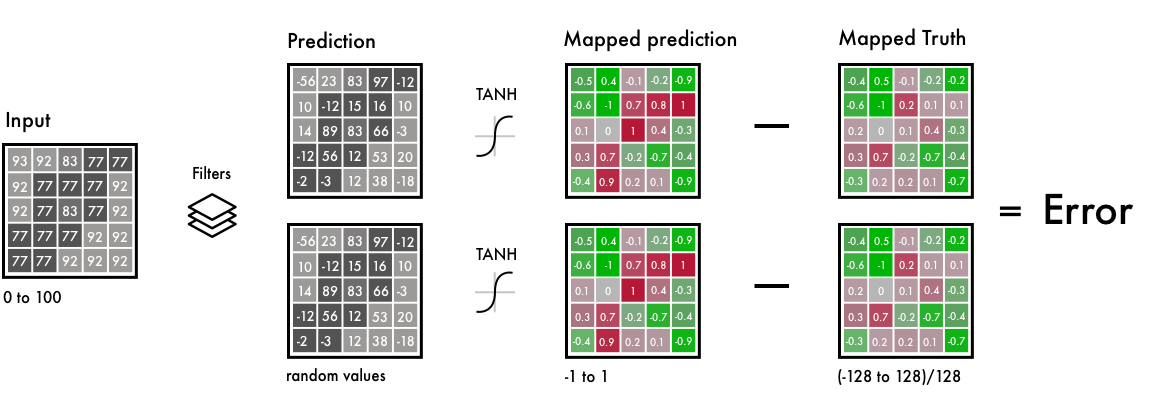
To the left side, we have the B&W input, or filters and the prediction from our neural network.

We map the predicted values and the real values within the same interval. This way, we can compare the values. The interval goes from -1 to 1. To map the predicted values we use a Tanh activation function. For any value you give the Tanh function, it will return -1 to 1.

The true color values go from -128 to 128, this is the default interval in the Lab color space. By dividing them with 128, they too fall within the -1 to 1 interval. This enables us to compare the error from our prediction.

After calculating the final error, the network updates the filters to reduce the total error. The network stays in this loop until the error is as low as possible.

Let’s clarify some syntax in the code snippet.

X = rgb2lab(1.0/255*image)[:,:,0]
Y = rgb2lab(1.0/255*image)[:,:,1:]

1.0/255, indicates that we are using a 24-bit RGB color space. It means that we are using 0-255 numbers for each color channel. This is the standard size of colors and results in 16.7 million color combinations. Since humans can only perceive 2-10 million colors, it does not make much sense to use a larger color space.

Y = Y / 128

The Lab color space has a different range compared to RGB. The color spectrum ab in Lab goes from -128 to 128. By dividing all values in the output layer with 128, we force the range between -1 and 1. We match it with our neural network, which also returns values between -1 and 1.

After converting the color space from rgb2lab(), we select the grayscale layer with: [:, :, 0]. This is our input for the neural network. [:, :, 1:] selects the two color layers green–red and blue–yellow.

After training the neural network, we make a final prediction which we convert into a picture.

output = model.predict(X)
output = output * 128

Here we use a grayscale image as input and run it through our trained neural network. We take all the output values between -1 and 1 and multiply it with 128. This gives us the correct color in the Lab color spectrum.

canvas = np.zeros((400, 400, 3))
canvas[:,:,0] = X[0][:,:,0]
canvas[:,:,1:] = output[0]

Lastly, we create a black RGB canvas by filling it with three layers of 0s. Then we copy the grayscale layer from our test image. Then we add our two color layers to the RGB canvas. This array of pixel values is then converted into a picture.

Takeaways from the Alpha version

• Reading research papers is painful. Once I summarized the core characteristics of each paper, it became easier to skim papers. It also allowed me to put the details into a context.
• Starting simple is key. Most of the implementations I could find online where 2-10K lines long. That made it hard to get an overview of the core logic of the problem. Once I had a barebone version it became easier to read code implementation, but also the research papers.
• Explore public projects. To get a rough idea for what to code, I skimmed 50-100 projects on colorization on Github.
• Things won't always work as expected. In the beginning, it could only create red and yellow colors. At first, I had a Relu activation function for the final activation. Since it only maps numbers into positive digits, it could not create negative values, the blue and green spectrums. Adding a Tanh activation function and mapping the Y values fixed this.
• Understanding > Speed. Many of the implementations I saw were fast but hard to work with. I chose to optimize for innovation speed instead of code speed.

The Beta Version

To understand the weakness of the Alpha-version, try coloring an image it has not been trained on. If you try it, you’ll see that it makes a poor attempt. It’s because the network has memorized the information. It has not learned how to color an image it hasn’t seen before. But this is what we’ll do in the Beta-version - we’ll teach our network to generalize.

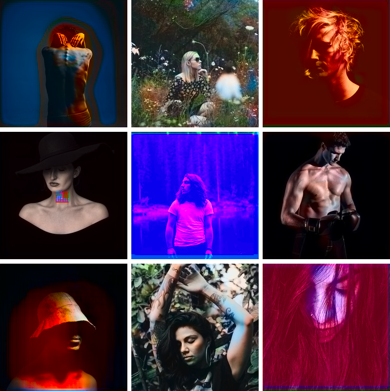
Below is the result of coloring the validation images with our Beta version.

Instead of using Imagenet, I created a public dataset on FloydHub with higher quality images. The images are from Unsplash - creative commons pictures by professional photographers. It includes 9.5 thousand training images and 500 validation images.

The feature extractor

Our neural network finds characteristics that link grayscale images with their colored versions.

Imagine you had to color black and white images - but with restriction that you can only see nine pixels at a time. You could scan each image from the top left to bottom right and try to predict which color each pixel should be.

For example, these nine pixels is the edge of the nostril from the woman just above. As you can imagine, it’d be next to impossible to make a good colorization, so you break it down into steps.

First, you look for simple patterns: a diagonal line, all black pixels, and so on. You look for the same exact pattern in each square and remove the pixels that don’t match. You generate 64 new images from your 64 mini filters.

If you scan the images again, you’d see the same small patterns you’ve already detected. To gain a higher level understanding of the image, you decrease the image size in half.

You still only have a three by three filter to scan each image. But by combining your new nine pixels with your lower level filters you can detect more complex patterns. One pixel combination might form a half circle, a small dot, or a line. Again, you repeatedly extract the same pattern from the image. This time, you generate 128 new filtered images.

After a couple of steps the filtered images you produce might look something like these:

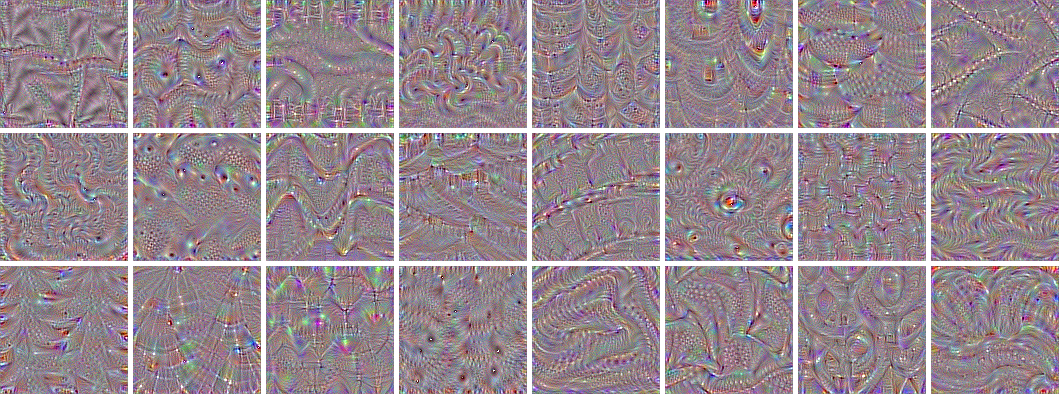
As mentioned, you start with low-level features, such as an edge. Layers closer to the output are combined into patterns, then into details, and eventually transformed into a face. If this is hard to grasp, then watch this video tutorial.

The process is like most neural networks that deal with vision, known as convolutional neural networks. Convolution is similar to the word combine, you combine several filtered images to understand the context in the image.

From feature extraction to color

The neural network operates in a trail and error manner. It first makes a random prediction for each pixel. Based on the error for each pixel, it works backward through the network to improve the feature extraction.

It starts adjusting for the situations that generate the largest errors. In this case, it’s whether to color or not and to locate different objects. Then it colors all the objects brown. It’s the color that is most similar to all other colors, thus producing the smallest error.

Because most of the training data is quite similar, the network struggles to differentiate between different objects. It will adjust different tones of brown, but fail to generate more nuanced colors. That’s what we’ll explore in the full version.

Below is the code for the beta-version, followed by a technical explanation of the code.

# Get images
X = []
for filename in os.listdir('../Train/'):
    X.append(img_to_array(load_img('../Train/'+filename)))
X = np.array(X, dtype=float)

# Set up training and test data
split = int(0.95*len(X))
Xtrain = X[:split]
Xtrain = 1.0/255*Xtrain

#Design the neural network
model = Sequential()
model.add(InputLayer(input_shape=(256, 256, 1)))
model.add(Conv2D(64, (3, 3), activation='relu', padding='same'))
model.add(Conv2D(64, (3, 3), activation='relu', padding='same', strides=2))
model.add(Conv2D(128, (3, 3), activation='relu', padding='same'))
model.add(Conv2D(128, (3, 3), activation='relu', padding='same', strides=2))
model.add(Conv2D(256, (3, 3), activation='relu', padding='same'))
model.add(Conv2D(256, (3, 3), activation='relu', padding='same', strides=2))
model.add(Conv2D(512, (3, 3), activation='relu', padding='same'))
model.add(Conv2D(256, (3, 3), activation='relu', padding='same'))
model.add(Conv2D(128, (3, 3), activation='relu', padding='same'))
model.add(UpSampling2D((2, 2)))
model.add(Conv2D(64, (3, 3), activation='relu', padding='same'))
model.add(UpSampling2D((2, 2)))
model.add(Conv2D(32, (3, 3), activation='relu', padding='same'))
model.add(Conv2D(2, (3, 3), activation='tanh', padding='same'))
model.add(UpSampling2D((2, 2)))

# Finish model
model.compile(optimizer='rmsprop', loss='mse')

# Image transformer
datagen = ImageDataGenerator(
        shear_range=0.2,
        zoom_range=0.2,
        rotation_range=20,
        horizontal_flip=True)

# Generate training data
batch_size = 50
def image_a_b_gen(batch_size):
    for batch in datagen.flow(Xtrain, batch_size=batch_size):
        lab_batch = rgb2lab(batch)
        X_batch = lab_batch[:,:,:,0]
        Y_batch = lab_batch[:,:,:,1:] / 128
        yield (X_batch.reshape(X_batch.shape+(1,)), Y_batch)

# Train model
TensorBoard(log_dir='/output')
model.fit_generator(image_a_b_gen(batch_size), steps_per_epoch=10000, epochs=1)
# Test images
Xtest = rgb2lab(1.0/255*X[split:])[:,:,:,0]
Xtest = Xtest.reshape(Xtest.shape+(1,))
Ytest = rgb2lab(1.0/255*X[split:])[:,:,:,1:]
Ytest = Ytest / 128
print model.evaluate(Xtest, Ytest, batch_size=batch_size)

# Load black and white images
color_me = []
for filename in os.listdir('../Test/'):
        color_me.append(img_to_array(load_img('../Test/'+filename)))
color_me = np.array(color_me, dtype=float)
color_me = rgb2lab(1.0/255*color_me)[:,:,:,0]
color_me = color_me.reshape(color_me.shape+(1,))

# Test model
output = model.predict(color_me)
output = output * 128

# Output colorizations
for i in range(len(output)):
        cur = np.zeros((256, 256, 3))
        cur[:,:,0] = color_me[i][:,:,0]
        cur[:,:,1:] = output[i]
        imsave("result/img_"+str(i)+".png", lab2rgb(cur))

Here’s the FloydHub command to run the Beta neural network:

floyd run --data emilwallner/datasets/colornet/2:data --mode jupyter --tensorboard

Technical Explanation

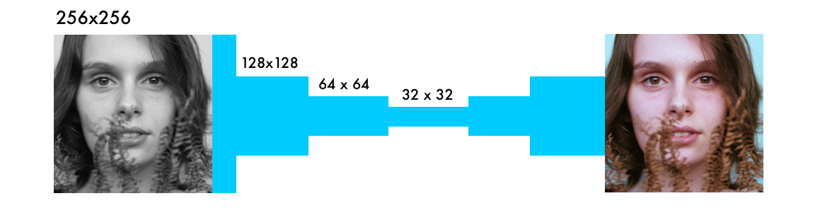
The main difference from other visual networks is the importance of pixel location. In coloring networks, the image size or ratio stays the same throughout the network. In other networks, the image gets distorted the closer it gets to the final layer.

The max-pooling layers in classification networks increase the information density, but also distort the image. It only values the information, but not the layout of an image. In coloring networks we instead use a stride of 2, to decrease the width and height by half. This also increases information density but does not distort the image.

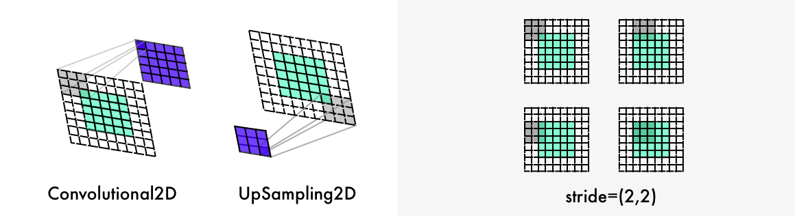
Two further differences are upsampling layers and maintaining the image ratio. Classification networks only care about the final classification. Therefore, they keep decreasing the image size and quality as it moves through the network.

Coloring networks keep the image ratio. This is done by adding white padding like the visualization above. Otherwise, each convolutional layer cuts the images. It’s done with the *padding='same'* parameter. **

To double the size of the image, the coloring network uses an upsampling layer. [Documentation]

for filename in os.listdir('/Color_300/Train/'):
    X.append(img_to_array(load_img('/Color_300/Test'+filename)))

This for loop first counts all the file names in the directory. Then, it iterates through the image directory, converts the images into an array of pixels, and combines them into a giant vector.

datagen = ImageDataGenerator(
        shear_range=0.2,
        zoom_range=0.2,
        rotation_range=20,
        horizontal_flip=True)

In the ImageDataGenerator, we adjust the setting for our image generator. This way, one image will never be the same, thus improving the learning. The shear_range tilts the image to the left or right, and the other settings should be self-explanatory. [Documentation]

batch_size = 50
def image_a_b_gen(batch_size):
    for batch in datagen.flow(Xtrain, batch_size=batch_size):
        lab_batch = rgb2lab(batch)
        X_batch = lab_batch[:,:,:,0]
        Y_batch = lab_batch[:,:,:,1:] / 128
        yield (X_batch.reshape(X_batch.shape+(1,)), Y_batch)

We use the images from our folder, Xtrain, generating images based on the settings above. Then we extract the black and white layer for the X_batch and the two colors for the two color layers.

model.fit_generator(image_a_b_gen(batch_size), steps_per_epoch=1, epochs=1000)

The stronger GPU you have the more images you can fit into it. With this setup, you can use 50-100 images. The steps_per_epoch is calculated by dividing the number of training images with your batch size. For example, 100 images with a batch size of 50, equal to 2 steps per epoch. The number of epochs determines how many times you want to train all images. 10K images with 21 epochs will take about 11 hours on a Tesla K80 GPU.

Takeaways

• Make a lot of experiments in smaller batches before you make larger runs. Even after 20-30 experiments, I still found mistakes. Just because it’s running doesn’t mean it’s working. Bugs in a neural network are often more nuanced than traditional programming errors. One of the more bizarre ones was my Adam hiccup.
• A more diverse dataset makes the pictures brownish. If you have very similar images, you can have a decent result without having a more complex architecture. But they also worse at generalizing.
• Shapes, shapes, and shapes. The size of each image has to be exact and remain proportional throughout the network. In the beginning, I used the image size 300, by dividing it in half three times you get 150, 75, and 35.5. Thus, losing half of a pixel. This led to many “hacks” until I realized it’s better to use a power of two: 2, 8, 16, 32, 64, 256 and so on.
• Creating datasets
  • Disable the .DS_Store file, it drove me crazy.
  • Be creative. I ended up with a Chrome console script and an extension to download the files.
  • Make a copy of the raw files you scrape and structure your cleaning scripts.

Full-version

Our final version of the colorization neural network has four components. We split the network we had before into an encoder and a decoder. Between them, we’ll use a fusion layer. If you are new to classification networks, I’d recommend having a quick glance at this tutorial.

In parallel to the encoder, the input images also run through one of the today’s most powerful classifiers — the inception resnet v2 — a network trained on 1.2M images. We extract the classification layer and merge it with the output from the encoder.

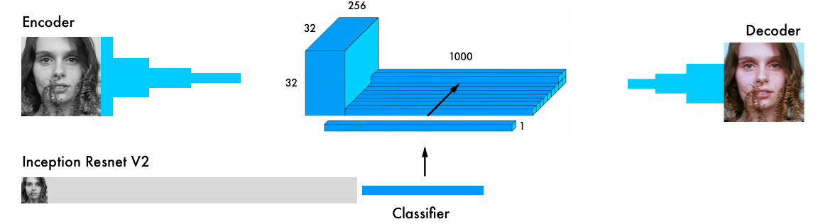
Here is a more detailed visual from the original paper.

By transferring the learning from the classifier to the coloring network, the network can get a sense of what’s in the picture. Thus, enabling the network to match an object representation with a coloring scheme.

Here are some of the validation images, using only 20 images to train the network on.

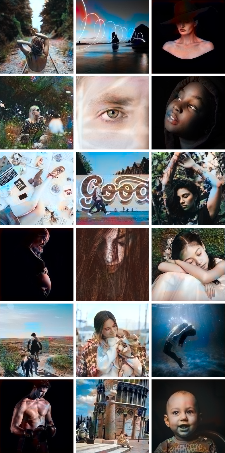
Most of the images turned out poor, but I managed to find a few decent ones because of a large validation set (2,500 images). Training it on more images gave a more consistent result, but most of them turned out brownish. Here is a full list of the experiments I ran including the validation images [1][2].

Here are the most common architectures from previous research:

Architectures

• Manually adding small dots of color in a picture to guide the neural network [1]
• Find a matching image and transfer the coloring [1][2][3]
• Residual encoder and merging classification layers [1]
• Merging hypercolumns from a classifying network [1][2]
• Merging the final classification between the encoder and decoder [1][2]

Colorspaces

Lab, YUV, HSV, and LUV [1][2][3][4]

Loss

Mean square error, classification, weighted classification [1][2][3]

I chose E, the one with the fusion layer. It has some of the best results and it’s easy to understand and reproduce in Keras. Although it’s not the strongest color network design, it’s ideal to start. It’s a great architecture to understand the dynamics of the coloring problem.

I used the neural network design from this paper (Baldassarre alt el., 2017), with my own interpretation in Keras.

Note: in the below code I switch from Keras’ sequential model to their functional API. [Documentation]

# Get images
X = []
for filename in os.listdir('/data/images/Train/'):
    X.append(img_to_array(load_img('/data/images/Train/'+filename)))
X = np.array(X, dtype=float)
Xtrain = 1.0/255*X

#Load weights
inception = InceptionResNetV2(weights=None, include_top=True)
inception.load_weights('/data/inception_resnet_v2_weights_tf_dim_ordering_tf_kernels.h5')
inception.graph = tf.get_default_graph()

embed_input = Input(shape=(1000,))

#Encoder
encoder_input = Input(shape=(256, 256, 1,))
encoder_output = Conv2D(64, (3,3), activation='relu', padding='same', strides=2)(encoder_input)
encoder_output = Conv2D(128, (3,3), activation='relu', padding='same')(encoder_output)
encoder_output = Conv2D(128, (3,3), activation='relu', padding='same', strides=2)(encoder_output)
encoder_output = Conv2D(256, (3,3), activation='relu', padding='same')(encoder_output)
encoder_output = Conv2D(256, (3,3), activation='relu', padding='same', strides=2)(encoder_output)
encoder_output = Conv2D(512, (3,3), activation='relu', padding='same')(encoder_output)
encoder_output = Conv2D(512, (3,3), activation='relu', padding='same')(encoder_output)
encoder_output = Conv2D(256, (3,3), activation='relu', padding='same')(encoder_output)

#Fusion
fusion_output = RepeatVector(32 * 32)(embed_input) 
fusion_output = Reshape(([32, 32, 1000]))(fusion_output)
fusion_output = concatenate([encoder_output, fusion_output], axis=3) 
fusion_output = Conv2D(256, (1, 1), activation='relu', padding='same')(fusion_output) 

#Decoder
decoder_output = Conv2D(128, (3,3), activation='relu', padding='same')(fusion_output)
decoder_output = UpSampling2D((2, 2))(decoder_output)
decoder_output = Conv2D(64, (3,3), activation='relu', padding='same')(decoder_output)
decoder_output = UpSampling2D((2, 2))(decoder_output)
decoder_output = Conv2D(32, (3,3), activation='relu', padding='same')(decoder_output)
decoder_output = Conv2D(16, (3,3), activation='relu', padding='same')(decoder_output)
decoder_output = Conv2D(2, (3, 3), activation='tanh', padding='same')(decoder_output)
decoder_output = UpSampling2D((2, 2))(decoder_output)

model = Model(inputs=[encoder_input, embed_input], outputs=decoder_output)

#Create embedding
def create_inception_embedding(grayscaled_rgb):
    grayscaled_rgb_resized = []
    for i in grayscaled_rgb:
        i = resize(i, (299, 299, 3), mode='constant')
        grayscaled_rgb_resized.append(i)
    grayscaled_rgb_resized = np.array(grayscaled_rgb_resized)
    grayscaled_rgb_resized = preprocess_input(grayscaled_rgb_resized)
    with inception.graph.as_default():
        embed = inception.predict(grayscaled_rgb_resized)
    return embed

# Image transformer
datagen = ImageDataGenerator(
        shear_range=0.4,
        zoom_range=0.4,
        rotation_range=40,
        horizontal_flip=True)

#Generate training data
batch_size = 20

def image_a_b_gen(batch_size):
    for batch in datagen.flow(Xtrain, batch_size=batch_size):
        grayscaled_rgb = gray2rgb(rgb2gray(batch))
        embed = create_inception_embedding(grayscaled_rgb)
        lab_batch = rgb2lab(batch)
        X_batch = lab_batch[:,:,:,0]
        X_batch = X_batch.reshape(X_batch.shape+(1,))
        Y_batch = lab_batch[:,:,:,1:] / 128
        yield ([X_batch, create_inception_embedding(grayscaled_rgb)], Y_batch)

#Train model      
tensorboard = TensorBoard(log_dir="/output")
model.compile(optimizer='adam', loss='mse')
model.fit_generator(image_a_b_gen(batch_size), callbacks=[tensorboard], epochs=1000, steps_per_epoch=20)

#Make a prediction on the unseen images
color_me = []
for filename in os.listdir('../Test/'):
    color_me.append(img_to_array(load_img('../Test/'+filename)))
color_me = np.array(color_me, dtype=float)
color_me = 1.0/255*color_me
color_me = gray2rgb(rgb2gray(color_me))
color_me_embed = create_inception_embedding(color_me)
color_me = rgb2lab(color_me)[:,:,:,0]
color_me = color_me.reshape(color_me.shape+(1,))


# Test model
output = model.predict([color_me, color_me_embed])
output = output * 128

# Output colorizations
for i in range(len(output)):
    cur = np.zeros((256, 256, 3))
    cur[:,:,0] = color_me[i][:,:,0]
    cur[:,:,1:] = output[i]
    imsave("result/img_"+str(i)+".png", lab2rgb(cur))

Here’s the FloydHub command to run the full neural network:

floyd run --data emilwallner/datasets/colornet/2:data --mode jupyter --tensorboard

Technical Explanation

Keras’s functional API is ideal when we are concatenating or merging several models.

First, we download the inception resnet v2 neural network and load the weights. Since we will be using two models in parallel we need to specify which model we are using. This is done in Tensorflow, the backend for Keras.

inception = InceptionResNetV2(weights=None, include_top=True)
inception.load_weights('/data/inception_resnet_v2_weights_tf_dim_ordering_tf_kernels.h5')
inception.graph = tf.get_default_graph()

To create our batch, we use the tweaked images. We turn them black and white and run in through the inception resnet model.

grayscaled_rgb = gray2rgb(rgb2gray(batch))
embed = create_inception_embedding(grayscaled_rgb)

First, we have to resize the image to fit into the inception model. Then we use the preprocessor to format the pixel and color values according to the model. In the final step, we run it through the inception network and extract the final layer of the model.

def create_inception_embedding(grayscaled_rgb):
    grayscaled_rgb_resized = []
    for i in grayscaled_rgb:
        i = resize(i, (299, 299, 3), mode='constant')
        grayscaled_rgb_resized.append(i)
    grayscaled_rgb_resized = np.array(grayscaled_rgb_resized)
    grayscaled_rgb_resized = preprocess_input(grayscaled_rgb_resized)
    with inception.graph.as_default():
        embed = inception.predict(grayscaled_rgb_resized)
    return embed

Going back to the generator. For each batch, we generate 20 images in the below format. It takes about an hour on a Tesla K80 GPU. It can do up to 50 images at a time with this model without having memory problems.

yield ([X_batch, create_inception_embedding(grayscaled_rgb)], Y_batch)

This matches with our colornet model format.

model = Model(inputs=[encoder_input, embed_input], outputs=decoder_output)

encoder_input is fed into our Encoder model, the output of the Encoder model is then fused with the embed_input in the fusion layer; the output of the fusion is then used as input in our Decoder model, which then returns the final output, decoder_output.

fusion_output = RepeatVector(32 * 32)(embed_input) 
fusion_output = Reshape(([32, 32, 1000]))(fusion_output)
fusion_output = concatenate([fusion_output, encoder_output], axis=3) 
fusion_output = Conv2D(256, (1, 1), activation='relu')(fusion_output)

In the fusion layer, we first multiply the 1000 category layer by 1024 (32 * 32). This way, we get 1024 rows with the final layer from the inception model. It’s then reshaped from 2D to 3D, a 32 x 32 grid with the 1000 category pillars. These are then linked together with the output from the encoder model. We apply a 254 filtered convolutional network with a 1X1 kernel, the final output of the fusion layer.

Takeaways

• The research terminology was daunting. I spent three days googling for ways to implement the “Fusion model” in Keras. Because it sounded complex, I didn’t want to face the problem. Instead, I tricked myself into searching for short cuts.
• I asked questions online. I didn’t have a single comment in the Keras slack channel and Stack Overflow deleted my questions. But, by publicly breaking down the problem to make it simple to answer, it forced me to isolate the error, taking me closer to a solution.
• Email people. Although forums can be cold, people care if you connect with them directly. Discussing color spaces over Skype with a researcher you don’t know is inspiring.
• After procrastinating on the fusion problem, I decided to build all the components before I stitched them together. Here are a few experiments I used to break down the fusion layer.
• Once I had something I thought would work, I was hesitant of running it. Although I knew the core logic was okay, I didn’t believe it would work. After a cup of lemon tea and a long walk — I ran it. It produced an error after the first line in my model. But after four days, several hundred bugs and several thousand Google searches, “Epoch 1/22” appeared under my model.

Next steps

Colorizing images is a deeply fascinating problem. It is as much as a scientific problem as artistic one. I wrote this article so you can get up to speed in coloring and continue where I left off. Here are some suggestions to get started:

• Implement it with another pre-trained model
• A different dataset
• Enable the network to grow in accuracy with more pictures
• Build an amplifier within the RGB color space. Create a similar model to the coloring network, that takes a saturated colored image as input and the correct colored image as output.
• Implement a weighted classification
• Use a classification neural network as a loss function. Pictures that are classified as fake produce an error. It then decides how much each pixel contributed to the error.
• Apply it to video. Don’t worry too much about the colorization, but make the switch between images consistent. You could also do something similar for larger images, by tiling smaller ones.

You can also easily colorize your own black and white images with my three versions of the colorization neural network using FloydHub.

• For the alpha version, simply replace the woman.jpg file with your file with the same name (image size 400x400 pixels).
• For the beta and the full version, add your images to the Test folder before you run the FloydHub command. You can also upload them directly in the Notebook to the Test folder while the notebook is running. Note that these images need to be exactly 256x256 pixels. Also, you can upload all test images in color because it will automatically convert them into B&W.

If you build something or get stuck, ping me on twitter: emilwallner. I’d love to see what you are building.

Huge thanks to Federico Baldassarre, for answering clarifying questions and their previous work on colorization. Also thanks to Muthu Chidambaram, which influenced the core implementation in Keras, the Unsplash community for providing the pictures. Also thanks to Marine Haziza, Valdemaras Repsys, Qingping Hou, Charlie Harrington, Sai Soundararaj, Jannes Klaas, Claudio Cabral, Alain Demenet, and Ignacio Tonoli for reading drafts of this.

Raising the bar

Ready to bring colorization to the next level?! Please, welcome DeOldify: A GAN-based approach to colorize and restore old images and movies.

FloydHub Call for AI writers

Want to write amazing articles like Emil and play your role in the long road to Artificial General Intelligence? We are looking for passionate writers, to build the world's best blog for practical applications of groundbreaking A.I. techniques. FloydHub has a large reach within the AI community and with your help, we can inspire the next wave of AI. Apply now and join the crew!

About Emil Wallner

This the third part in a multi-part blog series from Emil as he learns deep learning. Emil has spent a decade exploring human learning. He's worked for Oxford's business school, invested in education startups, and built an education technology business. Last year, he enrolled at Ecole 42 to apply his knowledge of human learning to machine learning. Emil is also an AI Writer for FloydHub.

You can follow along with Emil on Twitter and Medium.

We're always looking for more guests to write interesting blog posts about deep learning. Let us know on Twitter if you're interested.