Using Sentence Embeddings to Automate Customer Support, Part One
Most of your customer support questions have already been asked. Learn how to use sentence embeddings to automate your customer support with AI.


Most of your company's customer support questions have already been asked and answered.
You’re not alone, either. Amazon recently reported that up to 70% of their customer support responses were directly related to previous support answers.
But there’s hope yet — neural networks can be trained to identify semantic similarity among text, which you can directly apply to your customer support workflow. Imagine this:
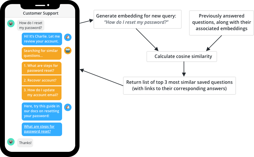
In this two-part blog post, we’ll develop a customer support workflow that can respond to incoming queries with a group of similar questions, making things a bit easier for your customer support agents.
Along the way, we’ll be diving headfirst into the world of embeddings. This post will introduce basic embedding concepts, including one-hot encodings and word embeddings. The second post will dig into the more recent concept of Universal Sentence Embeddings (USE) — and that’s also where we’ll put it all together with our demo customer support project.
Ready? Set. Embed.
A primer on embeddings
A core part of the deep learning approach to Natural Language Processing (NLP) tasks is the concept of an embedding.
In the context of NLP, when we’re talking about embeddings, what we are really talking about is vectors. And what's a vector, Victor? A vector is just a set of real numbers:
# v = [v1, v2, v3, .... ,vn]
# Where v1...vn are the real numbers or components of vector v

# For example:
v = [1, 3, 100, -30]
Importantly, we can use this set of real numbers to represent objects and phenomena in the world – such as a word or a sentence or even classical music.
What makes vectors different from a single real number is that they can also have a direction, which is a convenient feature that we'll exploit later on, when we start to identify similar vectors.
Why then have a different word for vector and embedding?
Well, an embedding refers to something that's been translated into a vector. This numerical representation as an array of numbers is useful because it facilitates a wide variety of mathematical operations.
For example, once we've created an embedding, we can locate this vector in something called a vector space. A vector space may sound like a difficult concept to grasp, but it’s simply a method to locate points in space. Here is an example:
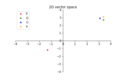
In our illustration above, we're plotting four points that represent four different two dimensional (2D) vectors along two dimensions. This vector space probably looks quite familiar to you – it resembles the traditional Cartesian X-Y plane.
Visualizing embeddings in a vector space helps us identify related entities. Let me explain. Let's assume that the vectors on the graph: P, Q, U and V each represent different sentence embeddings. We can easily see that Q, U and V are closely clustered together, whereas P is in an entirely different quadrant.
This simple form of visual clustering can be used to identify patterns and similar entities when we encode something as an embedding.
This approach does become more difficult at higher dimensions, but there are techniques which we can use to reduce the dimensions to 2 or 3 dimensions so that it becomes easier to identify these aspects.
Thus, embeddings facilitate our ability to perform mathematical operations on non-numeric things – and thereby enabled much of NLP.
But how we make an embedding? How many dimensions do we need? And how do we set the values for each dimension?
Excellent questions. Let's work through a simple example together, using a reduced vocabulary of only four words: king, queen, man, woman.
One-hot encoding: our first embedding technique
To recap, we want to create an embedding for each of the four words in our vocabulary – that is, we want to represent each word as a unique vector.
We'll use the technique called “one hot” encoding to embed our words into vectors. With one hot encoding, we'll identify a unique word in our vocabulary via one dimension (also known as a feature) of a vector. The size of each vector will be the total number of entities in our vocabulary.
Let's take a look at a "one hot" encoding of our four-word reduced vocabulary:
| King | Queen | Man | Woman | |
|---|---|---|---|---|
| King dimension | 1 | 0 | 0 | 0 |
| Queen dimension | 0 | 1 | 0 | 0 |
| Man dimension | 0 | 0 | 1 | 0 |
| Woman dimension | 0 | 0 | 0 | 1 |
Each column is an embedding, and each embedding has four dimensions (represented by the rows in this grid). You'll notice that each embedding only has one dimension that contains a 1 – the rest of its dimensions are 0.
Using the word King, you'll see that it has a 1 for the"King dimension" and a 0 for the rest. We can now use the vector [1,0,0,0] to in place of the word King.
We should also be able to see that we can expand this approach to any number of words by simply adding a new dimension for each new word in our vocabulary.
| King | Queen | Man | Woman | Joker | |
|---|---|---|---|---|---|
| King dimension | 1 | 0 | 0 | 0 | 0 |
| Queen dimension | 0 | 1 | 0 | 0 | 0 |
| Man dimension | 0 | 0 | 1 | 0 | 0 |
| Woman dimension | 0 | 0 | 0 | 1 | 0 |
| Joker dimension | 0 | 0 | 0 | 0 | 1 |
However, even without a deep understanding of vectors, we can probably already see see that this approach is wasteful. There will be lots of 0’s in our embeddings and the dimensionality will be very large. To use a more technical term in the industry, our embeddings will be very “sparsely” populated.
More importantly, our "one-hot" encoded embeddings tell us nothing about the relationships between the words in our reduced vocabulary set
As humans, we can easily discern that there is some connection between these words. “King” and “Queen” are both royal terms. “Man” and “Woman” are gender terms. But there is also a relationship between these pairs of terms. A “King” is traditionally associated with the word “Man” and a “Queen” is often associated with the word “Woman." Our one-hot encoding captures none of this relationship, however.
Visually representing embeddings
The easiest way to see these relationships is visually. In the previous section, our embeddings were only two dimensions in size, so it was easy to visually inspect them in a 2D vector space. But now we have four dimensional embeddings, so visual inspection becomes a bit more difficult. In the real world, we'll be dealing with hundreds of dimensions for our embeddings, so it's important to know how we can represent these visually in reduced dimensions.
Principal Component Analysis
To do this, we'll use a technique called Principal Component Analysis (PCA).
PCA is a way to identify the key information carrying parts of your embedding. It is trying to find out what is different and unique about each embedding, and will discard anything they have in common. PCA is a dimensional reduction technique (there are others such as T-SNE) which is used to highlight the important information in an embedding. We could spend much more time on PCA, but, for now, it is enough to just understand it is something we can use to reduce the dimensions of our embeddings.
Here's how we can plot our vocabulary using PCA using some basic Python machine learning libraries:
# Import the libraries
import numpy as np
import matplotlib.pyplot as plt
from sklearn.decomposition import PCA

# Use PCA to reduce the dimensions of the embedding
def pca_transform(arr1, arr2, arr3, arr4, dim):
    vectors = np.vstack((arr1, arr2, arr3, arr4))
    # Set the number of dimensions PCA will reduce to
    pca = PCA(n_components=dim)
    pca.fit(vectors)
    new_pca = pca.transform(vectors)
    print("original shape:   ", vectors.shape)
    print("transformed shape:", new_pca.shape)
    return(new_pca)

# Draw a 2d graph with the new dimensions
def two_d_graph(reduced_dims):
    colors = ("red", "green", "blue", "orange")
    groups = ("King", "Queen", "Man", "Woman")

    # Create plot
    fig = plt.figure()
    ax = fig.gca()

    for data, color, group in zip(reduced_dims, colors, groups):
        x, y = data
        ax.scatter(x, y, alpha=0.8, c=color, edgecolors='none', s=30, label=group)

    plt.title('Reduced vocab set')
    plt.legend(loc=1)
    plt.show()

# Transform the 4 dimensions to 2 via PCA
def vectors(a, b, c, d):
    emba = np.array(a)
    embb = np.array(b)
    embc = np.array(c)
    embd = np.array(d)
    new_dim = pca_transform(emba, embb, embc, embd, 2)
    two_d_graph(new_dim)

vectors([1,0,0,0], [0,1,0,0], [0,0,1,0], [0,0,0,1])
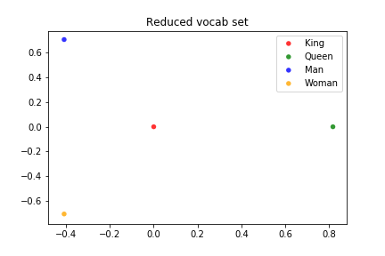
If you're struggling to find any clustering in this chart, that's totally expected! None of the points are clearly located together in terms of the other points. And this makes sense, if you think about it. Our embeddings carry no information about how words relate to each other. Since we can just keep arbitrarily adding dimensions for new words in vocabulary, there's nothing to tell us that one is closer to the other.
Nevertheless, "one hot" encoding is a valid embedding technique, since we've found a way to represent a word as a vector. But, clearly, we want to do more – and capture some of the connection between the words in our embeddings.
It's a useful exercise now to think about another set of words where one-hot encoding wouldn't capture some important context. Take a minute and think about it.
Okay, got one? Here's mine:
London
Washington, DC
Ireland
United Kingdom
United States
Can you see the connection? “Dublin”, “London” and “Washington D.C” are all in the "set" of capital cities, but they are also related to their respective countries. If we one-hot encode these all of this context will be lost.
We need to find some way to capture this context, and that is exactly what was achieved in 2013 with word embeddings.
Word embeddings: the power of context
Word2vec burst onto the scene in 2013 and entirely changed the NLP landscape, demonstrating that deep learning methods could yield incredible results when applied to NLP tasks such as translation, classification, and semantic parsing.
Word2vec, and similar approaches such as GloVe, showed that vector representations of words could be used to discover semantic meaning without requiring domain specific knowledge.
The key to these advances was finding a way to capture contextual information within an embedding. As we've seen, one-hot encoding makes it difficult to understand the relationship between words.
The British linguist J.R Firth believed that we could discover the features of a word by looking at the words around it. Or, as he more eloquently put it:
“You shall know a word by the company it keeps”
Essentially, you don’t need to know all the rules of grammar or even the dictionary definition of a word to understand it. Instead, you just need to see what other words it is used with. Then you can know whether it is similar to other words, since they may share the same “company,” as our old friend J.R. Firth would say.
| Words | Context |
|---|---|
| King and Man | He was a good King |
| King and Royalty | The King always wears a crown |
| King and Man | He lives like a King |
| Queen, King, Man, Woman | A Queen is the wife or widow of a King |
| Queen, Royalty and Woman | She was crowned Queen of England |
| Queen, King and Royalty | This is the palace the King and Queen live in. |
We can see from the table that the words “King”, “Queen”, “Man” and “Woman” are related since they often appear in the same sentences. While we might not explicitly use “Man” or “Woman” we get the context with words like “he” or “she” or “wife” and “husband”. All of this context provides clues as to how each word is related to each other.
Word2vec uses this idea to learn the context of words via deep learning. There are different forms of word2vec but the basic idea is that we train a neural network to learn the context of words. We feed it a lot of data (such as 1 million most commonly used words from 6 billion words in Google news corpus) and the network learns what words appear next to each other more frequently.
To store this context, the network creates vectors with slightly more dimensions than our earlier example. In most cases, there are around 300 dimensions (or features) to each embedding. They then use these word embeddings to identify similar groups or clusters of words.
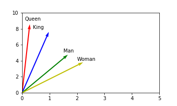
In the original Mikolov paper, they use the example of capital cities to show how this context has been learned.
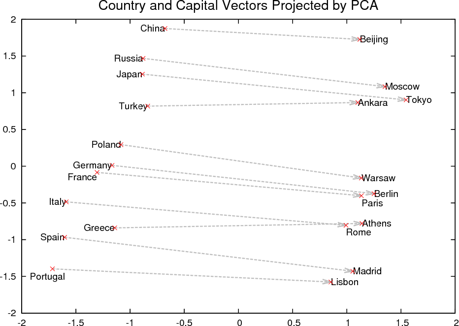
From the graph, we can see that all of the countries are clustered on the left while cities are on the right. So there seems to be a correlation between the words representing countries and, separately, a correlation between the words representing cities. But we also see that there is a correlation between each country and its capital city via a horizontal transformation, i.e. if we traverse the graph horizontally via the arrows we end up close to that country’s capital city and vice versa.
This did not happen by accident. We can imagine sentences in this dataset such as “Beijing is the capital of China” where these two words are commonly used together. And “Beijing has a population of X while Moscow has a population of Y”. Or “The top five most populated cities are …”
Normally, in order to learn this context, we would need to manually label all this data to train a network. We would manually tag a sentence to indicate it contains words for a capital city or a country for example. Then train the network with lots of examples.
But there are a number of problems with this approach:
- Firstly, the sheer volume of tagged data we would need would make it impractical.
- Secondly, how would we even know the tags to use for each word? Take a sentence like “Beijing is the capital of China”. We could tag it with “country” and “city” or “capital city”. We could also tag it as containing “geographic” related words. Or what about “location” or “municipality”? And this is a relatively simple collection of words in a short sentence. Tagging every word in a large corpus would be extremely difficult.
Deep learning neural networks help us identify features that we humans cannot see. While manual tagging would be better than one-hot encoding it would still be very limiting since we would need to identify all the features in advance. To address this problem word2vec used two approaches: skip-gram and Continuous Bag of Words (CBOW).
Skip-gram and CBOW enabled word2vec models to be trained without requiring any labelling of data. The key to both approaches is to use the context of the words in a sentence to train the network. The diagram shows the input and output for each method.
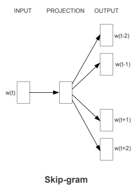
For skip-gram the input is a middle word in a sequence. The network then tries to predict the surrounding words
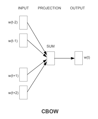
In CBOWs the input is the surrounding words and the network tries to predict the middle word. If the prediction is incorrect this is fed back to the network and the weights and bias are tweaked and the process continues until it can accurately predict the target word(s).
In this way, it uses the context of the words to train the network to recognize what words are commonly used together. If words appear together often, then they are likely to be related and the network will create embeddings which capture this information.
These embeddings will be far more advanced than our simple reduced vocabulary set. By visually inspecting them, as we did with our simple examples, we can begin to comprehend some of the magic hidden in our new embeddings.
A better King and Queen?
Earlier we created some embeddings using one-hot encoding and a vocabulary of four words. We saw that there was not much information contained in those embeddings. We did not learn anything new from those embeddings.
One of the surprising outcomes of the word2vec approach was that the generated embeddings encapsulated more information in the form of context than anyone thought possible. This was discovered by performing basic mathematical operations such as addition and subtraction on the generated embeddings.
The famous example used in the one of the early papers by Mikolov et al. was to manipulate the word embedding for “King” using algebra to generate an embedding close to “Queen”, i.e. King - Man + Woman = vector close to Queen.
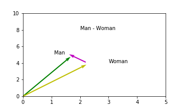
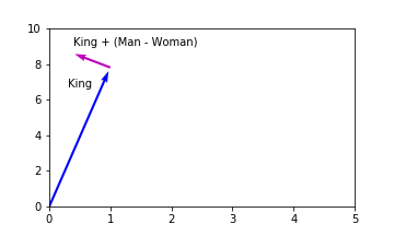
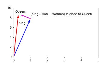
This was interesting since it provided some insight into what features may be represented by the dimensions of the embeddings. Being able to perform these types of operations implies that there are latent, hidden features of the embeddings which capture information relating to royalty and gender. For example, the dimensions might look something like:
This is different from our one-hot embeddings in a number of key ways:
- The values in the dimensions are not binary, they range from 0 to 1.
- Each word can have a value in more than one dimension
- The embeddings are not sparsely populated, there are very few 0’s.
If the dimensions of word embeddings contained something similar to the above table then the mathematical operations make sense. By subtracting the columns from each other we get transform the vectors to be close to other words in our vocabulary. Remember, this required no labelling of data in order to generate these embeddings. The neural network learned this context simply by looking at what words frequently appeared together or in close proximity in the data.
In this way, we can say that word embeddings are comprehensible – we can conceive of reasons why they work as they do.
Motivation for sentence embeddings
If word embeddings are so good at recognizing context, then why do we need sentence embeddings at all?
It’s a good question – and one that is open to significant debate. In short, we could use word embeddings as a proxy for a sentence embedding approach.
One simple way you could do this is by generating a word embedding for each word in a sentence, adding up all the embeddings and divide by the number of words in the sentence to get an “average” embedding for the sentence.
Alternatively, you could use a more advanced method which attempts to add a weighting function to word embeddings which down-weights common words. This latter approach is known as Smooth Inverse Frequency (SIF).
These methods can be used as a successful proxy for sentence embeddings. However, this “success” depends on the dataset being used and the task you want to execute. So for some tasks these methods could be good enough
However, there are a number of issues with any of these types of approaches:
- They ignore word ordering. So
your product is easy to use, I do not need any helpis identical toI do need help, your product is not easy to use. This is obviously problematic. - It's difficult to capture the semantic meaning of a sentence. The word crash can be used in multiple contexts, e.g.
I crashed a party,the stock market crashed, orI crashed my car. It’s difficult to capture this change of context in a word embedding. - Sentence length becomes problematic. With sentences we can chain them together to create a long sentence without saying very much,
The Philadelphia Eagles won the Super Bowl,The Washington Post reported that the Philadelphia Eagles won the Super Bowl,The politician claimed it was fake news when the Washington Post reported that the Philadelphia Eagles won the Super Bowl, and so on. All these sentences are essentially saying the same thing but if we just use word embeddings, it can be difficult to discover if they are similar. - They introduce extra complexity. When using word embeddings as a proxy for sentence embeddings we often need to take extra steps in conjunction with the base model. For example, we need to remove stop words, get averages, measure sentence length and so on.
Preview of part two: sentence embeddings
Can sentence embeddings address these shortcomings and provide an easy to use method for identifying sentence similarity?
In part two, we’ll investigate how much information we can pack into a single embedding. What happens when there are small changes in a sentence structure such as ordering or minor word changes? If sentence embeddings are such a new technology, can we know enough about them to put them into production?
To do this, we’ll evaluate sentence embeddings against a baseline of sentences from a Quora question database and build a simple customer support recommender system to show how they could be used in a typical customer support workflow.
About Cathal Horan
This is part one of a two-part blog series by Cathal Horan on sentence embeddings.
Cathal is interested in the intersection of philosophy and technology. Specifically how technologies such as deep learning can help augment and improve human decision making. He recently completed an MSc in Business Analytics. His primary degree is in electrical and electronic engineering. He also has a degree in philosophy and a MPhil in psychoanalytic studies. He currently works at Intercom. Cathal is also a FloydHub AI Writer.
You can follow along with Cathal on Twitter, and also on the Intercom blog.