A Pirate's Guide to Accuracy, Precision, Recall, and Other Scores
Once you've built your classifier, you need to evaluate its effectiveness with metrics like accuracy, precision, recall, F1-Score, and ROC curve.


Whether you're inventing a new classification algorithm or investigating the efficacy of a new drug, getting results is not the end of the process. Your last step is to determine the correctness of the results. There are a great number of methods and implementations for this task. Like many aspects of data science, there is no single best measurement for results quality; the problem domain and data in question determine appropriate approaches.
That said, there are a few measurements that are commonly introduced thanks to their conceptual simplicity, ease of implementation, and wide usefulness. Today, we will discuss seven such measurements:
- Confusion Matrix
- Accuracy
- Precision
- Recall
- Precision-Recall Curve
- F1-Score
- Area Under the Curve (AUC)
With these methods in your arsenal, you will be able to evaluate the correctness of most results sets across most domains.
One important thing to consider is the type of algorithm that is giving these results. Each of these metrics is designed for the output of a (binary) classification algorithm. These outputs have a number of records, and for each record there will be a "true" or "false" classification. However, we will discuss how to extend these measurements to other types of output where appropriate.
Briefly, a classification algorithm takes some input set and, for each member of the sets, classifies it as one of a fixed set of outputs. Examples of classification include facial recognition (match or not match), spam filters, and other kinds of pattern recognition with categorical output. Binary classification is a type of classification where there are only two possible outputs. An example of binary classification comes from perhaps the most famous educational data set in data science: the Titanic passenger dataset, where the binary outcome is survival of the disastrous sinking.


Finally, a quick note on syntax. The code samples in this article make heavy use of list comprehension with [function(element) for element in list if condition]. I use this syntax for its concision. If you are unfamiliar with this syntax, here is a resource. Otherwise, I tend to be explicit in my implementations, much shorter implementations of the following functions are trivial to construct.
Seven Metrics for the Seven Seas
While we will implement these measurements ourselves, we will also use the popular sklearn library to perform each calculation. Generally, it is best to use an established library like sklearn to perform standard operations such as these as the library's code is optimized, tested, and easy to use. This saves you time and ensures higher code quality, letting you focus on the differentiating aspects of your data science project.
For this article, we'll be exploring a variety of metrics and several example output sets. You can follow along on FloydHub's data science platform by clicking the link below.

Let's start with defining an extremely simple example binary dataset. Imagine, for a moment, that you are a pirate instead of a programmer. Furthermore, imagine that you have a device that purports to identify whether a ship on the horizon is carrying treasure, and that the device came with the data that we synthesized earlier. In this example, a "1" or positive identifies a ship with treasure (💰), and a "0" or negative identifies a ship without treasure (🧦). We'll use this example throughout the article to give meaning to the metrics.
# Setup A
actual_a = [1 for n in range(10)] + [0 for n in range(10)]
predicted_a = [1 for n in range(9)] + [0, 1, 1] + [0 for n in range(8)]
print(actual_a)
print(predicted_a)
| X | Raid-1 | Raid-2 | Raid-3 | Raid-4 | Raid-5 | Raid-6 | Raid-7 | Raid-8 | Raid-9 | Raid-10 | Raid-11 | Raid-12 | Raid-13 | Raid-14 | Raid-15 | Raid-16 | Raid-17 | Raid-18 | Raid-19 | Raid-20 |
|---|---|---|---|---|---|---|---|---|---|---|---|---|---|---|---|---|---|---|---|---|
| Actual | 💰 | 💰 | 💰 | 💰 | 💰 | 💰 | 💰 | 💰 | 💰 | 💰 | 🧦 | 🧦 | 🧦 | 🧦 | 🧦 | 🧦 | 🧦 | 🧦 | 🧦 | 🧦 |
| Predicted | 💰 | 💰 | 💰 | 💰 | 💰 | 💰 | 💰 | 💰 | 💰 | 🧦 | 💰 | 💰 | 🧦 | 🧦 | 🧦 | 🧦 | 🧦 | 🧦 | 🧦 | 🧦 |
This only produces 20 results. Statisticians debate about the fewest number of results needed for a conclusion to be, well, conclusive, but I wouldn't want to use fewer than 20. The number of results is of course domain and problem dependent, but in this case these 20 fake results will be enough to demonstrate the various metrics.
Confusion Matrix
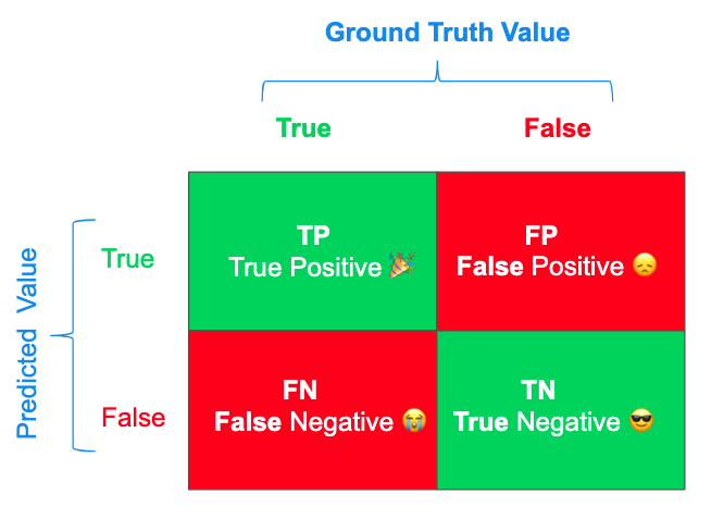
A holistic way of viewing true and false positive and negative results is with a confusion matrix. Despite the name, it is a straightforward table that provides an intuitive summary of the inputs to the calculations that we made above. Rather than a decimal correctness, the confusion matrix gives us counts of each of the types of results.
# Confusion Matrix
from sklearn.metrics import confusion_matrix

def my_confusion_matrix(actual, predicted):
    true_positives = len([a for a, p in zip(actual, predicted) if a == p and p == 1])
    true_negatives = len([a for a, p in zip(actual, predicted) if a == p and p == 0])
    false_positives = len([a for a, p in zip(actual, predicted) if a != p and p == 1])
    false_negatives = len([a for a, p in zip(actual, predicted) if a != p and p == 0])
    return "[[{} {}]\n  [{} {}]]".format(true_negatives, false_positives, false_negatives, true_positives)

print("my Confusion Matrix A:\n", my_confusion_matrix(actual_a, predicted_a))
print("sklearn Confusion Matrix A:\n", confusion_matrix(actual_a, predicted_a))
This yields the following table:
[[8 2]
 [1 9]]
Where the numbers correspond to:
[[true_negatives false_positives]
 [false_negatives true_positives]]
While there is no analytic conclusion in a confusion matrix, they are useful for two reasons. The first is that it is a concise visual representation of the absolute counts of correct and incorrect output. Furthermore, the confusion matrix introduces us to the four building blocks of our other metrics.
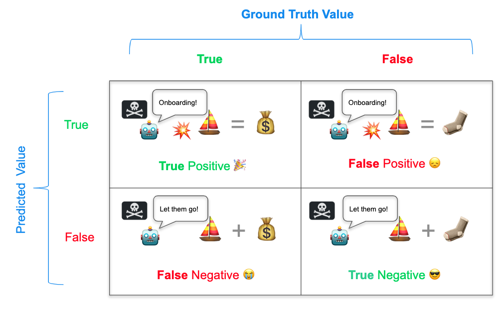
We're back on the pirate ship and evaluating the test results that came with the treasure-seeking device. In this case:
- A "True Positive" (TP), is when the device correctly identifies that a ship is carrying treasure. You raid the ship and share plunder among the crew.
- A "False Positive" (FP) is when the device says that a ship has treasure but it is empty. You raid the ship and the crew stages a mutiny over the disappointment of finding it empty.
- A "False Negative" (FN) is when the device says that a ship does not have treasure but it actually does. You let the ship pass, but when you get back to port the crew hears of another ship taking the bounty and some defect to the more successful crew.
- A "True Negative" (TN) is when the device correctly identifies that the ship is devoid of treasure. Your crew saves their strength as you let the ship pass.
Obviously, you want to maximize acquired treasure and minimize crew frustration. Should you use the device? We will calculate metrics to help you make an informed decision.
Accuracy
$$Accuracy = \dfrac{True\space Positive + True\space Negative}{True\space Positive + True\space Negative + False\space Positive + False\space Negative}$$
$$Accuracy = \dfrac{Ships\space carrying\space treasures\space correctly\space identified + Ships\space without\space treasures\space correctly\space identified}{All\space types\space of\space raid}$$
After synthesizing this data, our first metric is accuracy. Accuracy is the number of correct predictions over the output size. It is an incredibly straightforward measurement, and thanks to its simplicity it is broadly useful. Accuracy is one of the first metrics I calculate when evaluating results.
# Accuracy
from sklearn.metrics import accuracy_score

# Accuracy = TP + TN / TP + TN + FP + FN
def my_accuracy_score(actual, predicted): #threshold for non-classification?
    true_positives = len([a for a, p in zip(actual, predicted) if a == p and p == 1])
    true_negatives = len([a for a, p in zip(actual, predicted) if a == p and p == 0])
    false_positives = len([a for a, p in zip(actual, predicted) if a != p and p == 1])
    false_negatives = len([a for a, p in zip(actual, predicted) if a != p and p == 0])
    return (true_positives + true_negatives) / (true_positives + true_negatives + false_positives + false_negatives)

print("my Accuracy A:", my_accuracy_score(actual_a, predicted_a))
print("sklearn Accuracy A:", accuracy_score(actual_a, predicted_a))
The accuracy on this output is .85, which means that 85% of the results were correct. Note that, on average, random results yield an accuracy of 50%, so this is a major improvement (of course, this data is fabricated, but the point stands). This seems pretty good! Your crew will only doubt your leadership 15% of the time. That said, a mutiny at sea is worse than a grumbling on the docks, so you are right to be more concerned about false positives. Fortunately, another metric, precision, can help.
Precision
$$Precision = \dfrac{True\space Positive}{True\space Positive + False\space Positive}$$
$$Precision = \dfrac{Ships\space carrying\space treasures\space correctly\space identified}{Ships\space carrying\space treasures\space correctly\space identified + Ships\space incorrectly\space labeled\space as\space carrying\space treasures}$$
Precision is a similar metric, but it only measures the rate of false positives. In certain domains, like spam detection, a false positive is a worse error than a false negative (generally, missing an important email is worse than the inconvenience of deleting a piece of spam that snuck through the filter).
# Precision
from sklearn.metrics import precision_score

# Precision = TP / TP + FP
def my_precision_score(actual, predicted):
    true_positives = len([a for a, p in zip(actual, predicted) if a == p and p == 1])
    false_positives = len([a for a, p in zip(actual, predicted) if a != p and p == 1])
    return true_positives / (true_positives + false_positives)

print("my Precision A:", my_precision_score(actual_a, predicted_a))
print("sklearn Precision A:", precision_score(actual_a, predicted_a))
Our precision is approximately .818, lower than our accuracy. This means that false positives are a larger part of our error set. Indeed, we have two false positives in this example and only one false negative. This does not bode well for your career as a pirate captain if nearly one in five raids end in mutiny! However, for a more warlike crew, the disappointment of missing out on a raid might outweigh the cost of a pointless boarding. In such a situation, you would want to optimize for recall to reduce false negatives.
Recall
$$Recall = \dfrac{True\space Positive}{True\space Positive + False\space Negative}$$
$$Recall = \dfrac{Ships\space carrying\space treasures\space correctly\space identified}{Ships\space carrying\space treasures\space correctly\space identified + Ships\space carrying\space treasures\space incorrect\space classified\space as\space ships\space without\space treasures}$$
Recall is the opposite of precision, it measures false negatives against true positives. False negatives are especially important to prevent in disease detection and other predictions involving safety.
# Recall
from sklearn.metrics import recall_score

def my_recall_score(actual, predicted):
    true_positives = len([a for a, p in zip(actual, predicted) if a == p and p == 1])
    false_negatives = len([a for a, p in zip(actual, predicted) if a != p and p == 0])
    return true_positives / (true_positives + false_negatives)

print("my Recall A:", my_recall_score(actual_a, predicted_a))
print("sklearn Recall A:", recall_score(actual_a, predicted_a))
Our recall is .9, higher than the other two metrics. If we are especially concerned with reducing false negatives, then this is the best result. As a captain using your device, you are only letting one in ten ships pass by with their treasure holds intact.
Precision - Recall Curve
A precision-recall curve is a great metric for demonstrating the tradeoff between precision and recall for unbalanced datasets. In an unbalanced dataset, one class is substantially over-represented compared to the other. Our dataset is fairly balanced, so a precision-recall curve isn’t the most appropriate metric, but we can calculate it anyway for demonstration purposes.
#Precision-Recall
from sklearn.metrics import precision_recall_curve
import matplotlib.pyplot as plt

precision, recall, _ = precision_recall_curve(actual_a, predicted_a)
plt.step(recall, precision, color='g', alpha=0.2, where='post')
plt.fill_between(recall, precision, alpha=0.2, color='g', step='post')
plt.xlabel('Recall')
plt.ylabel('Precision')
plt.ylim([0.0, 1.0])
plt.xlim([0.0, 1.0])
plt.title('Precision-Recall curve')
plt.show()
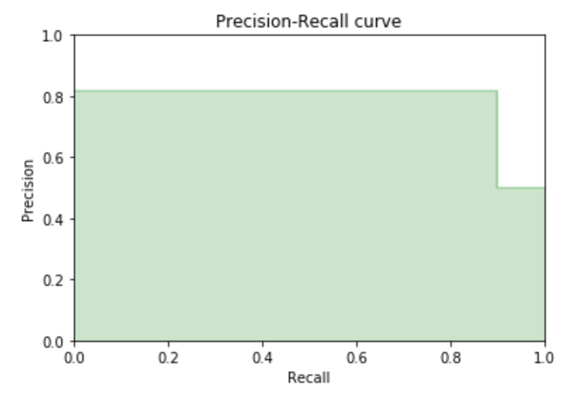
Our precision and recall are pretty similar, so the curve isn’t especially dramatic. Again, this metric is better suited to unbalanced classifiers.
F1-Score
$$F1-Score = 2 * \dfrac{Recall * Precision}{Recall + Precision}$$
What if you want to balance the two objectives: high precision and high recall? Or, as a pirate captain, you want to optimize towards capturing treasure and avoiding mutiny? We calculate the F1-score as the harmonic mean of precision and recall to accomplish just that. While we could take the simple average of the two scores, harmonic means are more resistant to outliers. Thus, the F1-score is a balanced metric that appropriately quantifies the correctness of models across many domains.
# F1 Score
from sklearn.metrics import f1_score

# Harmonic mean of (a, b) is 2 * (a * b) / (a + b)
def my_f1_score(actual, predicted):
    return 2 * (my_precision_score(actual, predicted) * my_recall_score(actual, predicted)) / (my_precision_score(actual, predicted) + my_recall_score(actual, predicted))

print("my F1 Score A:", my_f1_score(actual_a, predicted_a))
print("sklearn F1 Score A:", f1_score(actual_a, predicted_a))
The score of .857, slightly above that of the average, may or may not give you the confidence to rely on the device to help you decide which ships to raid. In evaluating the tradeoffs between precision and recall, you might want to draw an ROC curve on the back of one of the maps on the navigation deck.
Area Under the Curve
Unlike precision-recall curves, ROC (Receiver Operator Characteristic) curves work best for balanced data sets such as ours. Briefly, AUC is the area under the ROC curve that represents the tradeoff between Recall (TPR) and Specificity (FPR). Like the other metrics we have considered, AUC is between 0 and 1, with .5 as the expected value of random prediction. If you are interested in learning more, there is a great discussion on StackExchange as usual. Sklearn provides an implementation for AUC on binary classification.

The relevant equations are as follows:
$$True\space Positive\space Rate\space (a.k.a.\space Recall\space or\space Sensitivity) = \dfrac{True\space Positive}{True\space Positive + False Negative}$$
Refer back to the section on recall for this one; the TPR and recall are equivalent metrics.
$$False\space Positive\space Rate\space (a.k.a.\space Specificity) = \dfrac{False\space Positive}{False\space Positive + True\space Negative}$$
$$False\space Positive\space Rate = \dfrac{Ships\space without \space treasures\space incorrect\space classified\space as\space ships\space carrying\space treasures}{Ships\space without \space treasures\space incorrect\space classified\space as\space ships\space carrying\space treasures + Ships\space carrying\space treasures\space incorrect\space classified\space as\space ships\space without\space treasures}$$
The specificity or FPR of a classifier is its “false alarm metric.” Basically, it measures the frequency at which the classifier “cries wolf,” or predicts a positive where a negative is observed. In our example, a false positive is grounds for mutiny and should be avoided at all costs.
We consider the tradeoff between TPR and FPR with our ROC curve for our balanced classifier.
#ROC
from sklearn.metrics import roc_auc_score
from sklearn.metrics import roc_curve
import matplotlib.pyplot as plt

print("sklearn ROC AUC Score A:", roc_auc_score(actual_a, predicted_a))
fpr, tpr, _ = roc_curve(actual_a, predicted_a)
plt.figure()
plt.plot(fpr, tpr, color='darkorange',
         lw=2, label='ROC curve')
plt.plot([0, 1], [0, 1], color='navy', lw=2, linestyle='--') #center line
plt.xlim([0.0, 1.0])
plt.ylim([0.0, 1.05])
plt.xlabel('False Positive Rate')
plt.ylabel('True Positive Rate')
plt.title('Receiver operating characteristic example')
plt.legend(loc="lower right")
plt.show()
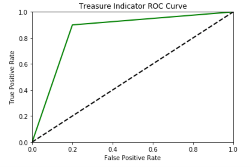
The AUC for our data is .85, which happens to be the same as our accuracy, which is not often the case (“see: balanced accuracy”). Again, this is a metric that balances the risks of the crew deserting and mutinying given the performance of our device to identify ships carrying treasures, and a ROC curve carved into the table of the navigator’s table could help you make your raiding decisions.
Because standard precision and recall rely on binary classification, it is non-trivial to extend AUC to represent a multidimensional general classifier as some sort of hypervolume-under-the-curve. However, several of the metrics are more straightforward to extend to evaluating other types of predictions.
Other Output Types
As I mentioned earlier, we can perform minor adaptations to these metrics to measure the performance of different types of output. We'll consider the simplest metric, accuracy, for both non-binary categorical output and continuous output.
In the following examples, an updated version of the device, version B, tells you if a ship has no treasure (0), some treasure (1), or tons of treasure (2). Version C of the device tells you how many islands you can buy with the treasure on the target ship.
For general categorical output, accuracy is very straightforward: correct_predictions/all_predictions. Using an example output with three categories, we can still determine the accuracy. In code, this looks like the following.
# Accuracy for non-binary predictions
def my_general_accuracy_score(actual, predicted):
    correct = len([a for a, p in zip(actual, predicted) if a == p])
    wrong = len([a for a, p in zip(actual, predicted) if a != p])
    return correct / (correct + wrong)

print("my Accuracy B:", my_general_accuracy_score(actual_b, predicted_b))
print("sklearn Accuracy B:", accuracy_score(actual_b, predicted_b))
As you may "recall," precision and recall measure false positives and negatives. With a bit of intuition and domain knowledge, we can extend this to a general classifier. In example B, I decided that "2" represents a positive and was able to generate precision as follows.
def my_general_precision_score(actual, predicted, value):
    true_positives = len([a for a, p in zip(actual, predicted) if a == p and p == value])
    false_positives = len([a for a, p in zip(actual, predicted) if a != p and p == value])
    return true_positives / (true_positives + false_positives)

print("my Precision B:", my_general_precision_score(actual_b, predicted_b, 2))
While sklearn supports accuracy for general categorical predictions, we can add a threshold parameter to calculate accuracy for a continuous prediction. Choosing the threshold is as important as every other number that you set during the modeling process, and should be set based on your domain knowledge before you see the results. After applying the threshold, the predictions can be treated a binary classifier and any of the seven metrics we have covered now apply to the data.
# Accuracy for continuous with threshold
def my_threshold_accuracy_score(actual, predicted, threshold):
    a = [0 if x >= threshold else 1 for x in actual]
    p = [0 if x >= threshold else 1 for x in predicted]
    return my_accuracy_score(a, p)

print("my Accuracy C:", my_threshold_accuracy_score(actual_c, predicted_c, 5))
Departing from the standard implementations gives us room to expand these fundamental metrics to cover most predictions, allowing for consistent comparison between models and their outputs.
Conclusion
These seven metrics for (binary) classification and continuous output with a threshold will serve you well for most data sets and modeling techniques. For the rest, minimal adjustments can create strong metrics. A single note of caution before we discuss adapting these standard measurements: always determine your evaluation criteria before beginning to evaluate the results. There are many subtle issues in a modeling process that can lead to overfitting and bad models, but adjusting the correctness evaluation metric based on the results of the model is an egregious departure from the accepted principles of a modeling workflow and will almost certainly promote overfitting and other bad results. Remember, accuracy is not the goal, a good model is the goal.
That goal is just a corollary of Goodhart’s law, or the idea that “when a measure becomes a target, it ceases to be a good measure..” Especially when you’re developing new systems, optimizations for individual metrics can hide overarching issues in the system. Rachel Thomas writes more about this, saying “I am not opposed to metrics; I am alarmed about the harms caused when metrics are overemphasized, a phenomenon that we see frequently with AI, and which is having a negative, real-world impact.”
There are extensions of classification that permit interesting modification to correctness metrics. For example, ordinal classification involves an output set where there are a fixed number of distinct categories, but those categories have a set order. Military rank is one type of ordinal data. Sometimes, you can handle ordinal data like continuous data and establish a threshold, then use a binary algorithm to handle the correctness. If a lieutenant in an army wanted to know if soldiers in a dataset were predicted to be her rank and above, she could set the cutoff at lieutenant and use a standard metric like accuracy or precision to evaluate the correctness of her prediction method.
However, a more generalized version of the same evaluation could use weighted accuracy to check the results. If a soldier is predicted to be a captain but he is in fact a sergeant, that is more incorrect than if he were predicted to be a lieutenant. Such disparity can be recognized in a custom implementation of accuracy or any other metric as appropriate for the domain, or by adding a penalty function to the loss function in the model.
Ultimately, I think this is what makes data science so interesting, there are opportunities to create custom solutions from the beginning to the end of the modeling process. However, the more non-standard the data and algorithm used, the more important it is to consider standard, fundamental metrics like accuracy, precision, and recall for evaluating the results. By using or adapting these metrics you can have confidence that your novel approach to a problem is correct with respect to standard practices.
Further References
- sklearn: confusion matrix
- sklearn: accuracy
- sklearn: precision
- sklearn: recall
- sklearn: precision-recall
- sklearn: f1-score
- sklearn: AUC
- sklearn: ROC
About Philip Kiely
Philip Kiely writes code and words. He is the author of Writing for Software Developers (2020). Philip holds a B.A. with honors in Computer Science from Grinnell College. Philip is a FloydHub AI Writer. You can find his work at https://philipkiely.com or you can connect with Philip via LinkedIn and GitHub.